Three (Rs) Tips for Better Statistical Analysis
Live demonstration
Ooh! Risky!
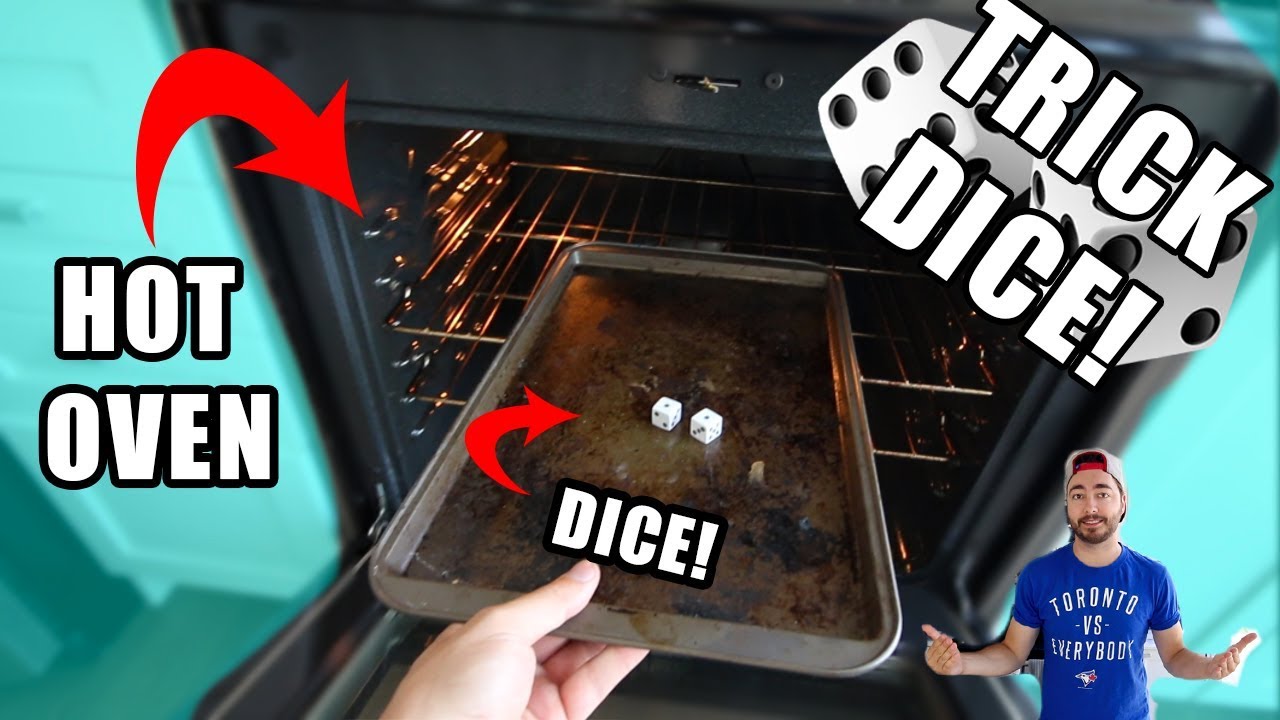
Figure 1: How to bias dice by heating them in an oven at about 121degC for 10min. Don’t use a microwave or blame me for the consequences/if you get caught.
Simulation: 1000 rolls
Use NC3Rs EDA
Please share the EDA diagram/session with your statistician.
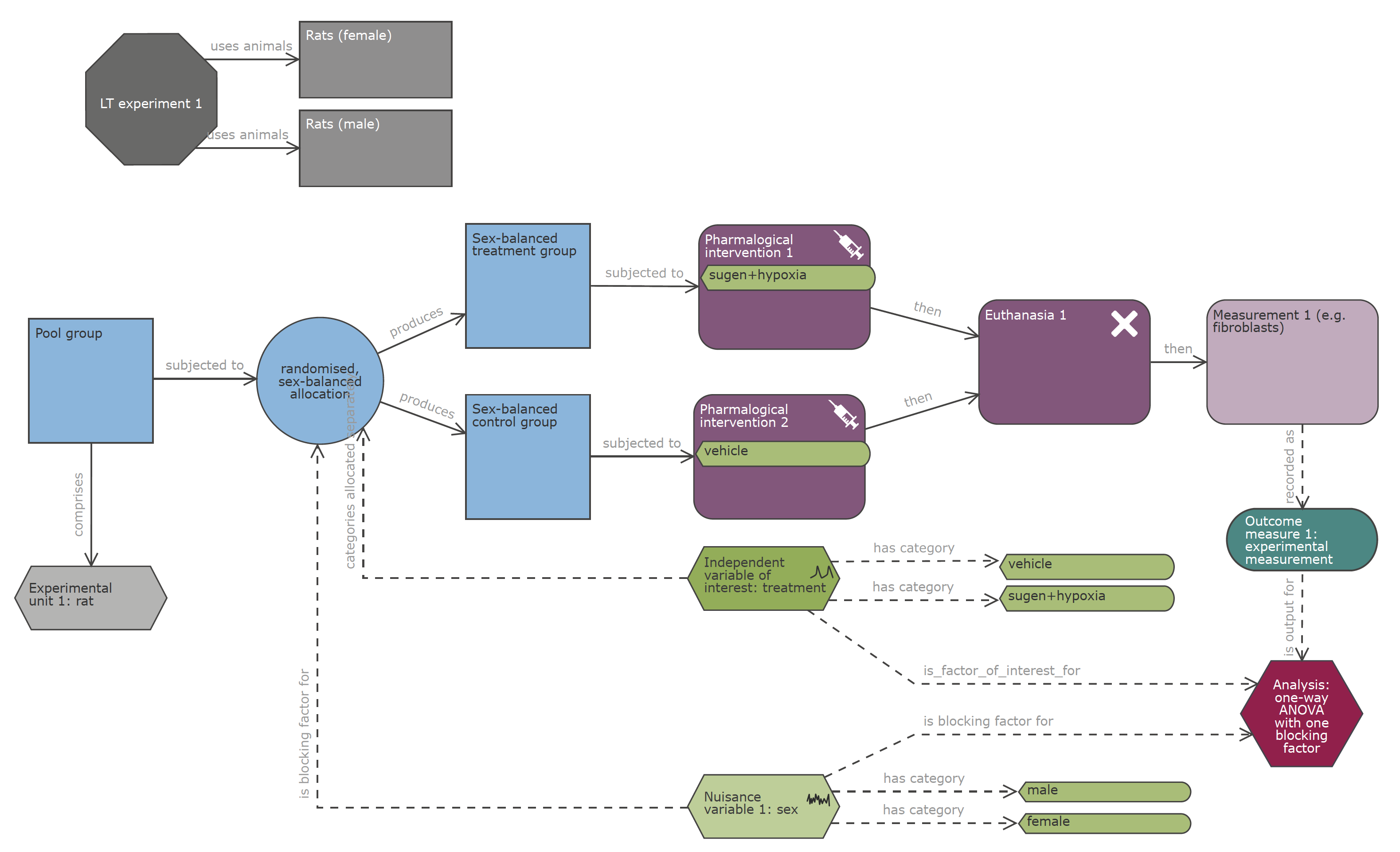
Figure 2: NC3Rs EDA forces clarification of concepts and is a focus for discussion.
An experimental dataset
- A control (
ctrl) and two treatments (trt1,trt2)
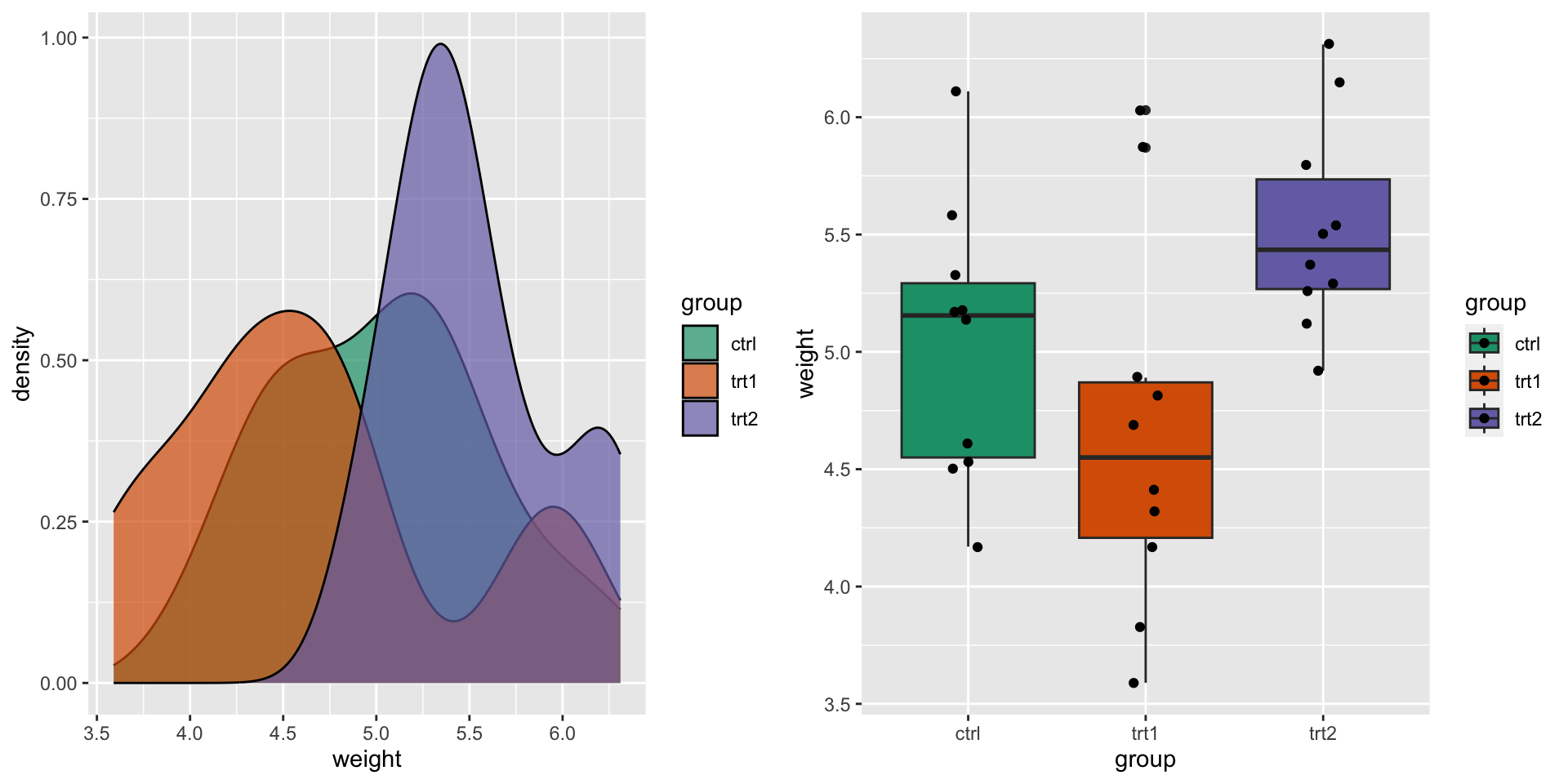
- Does it look like there are differences between the groups?
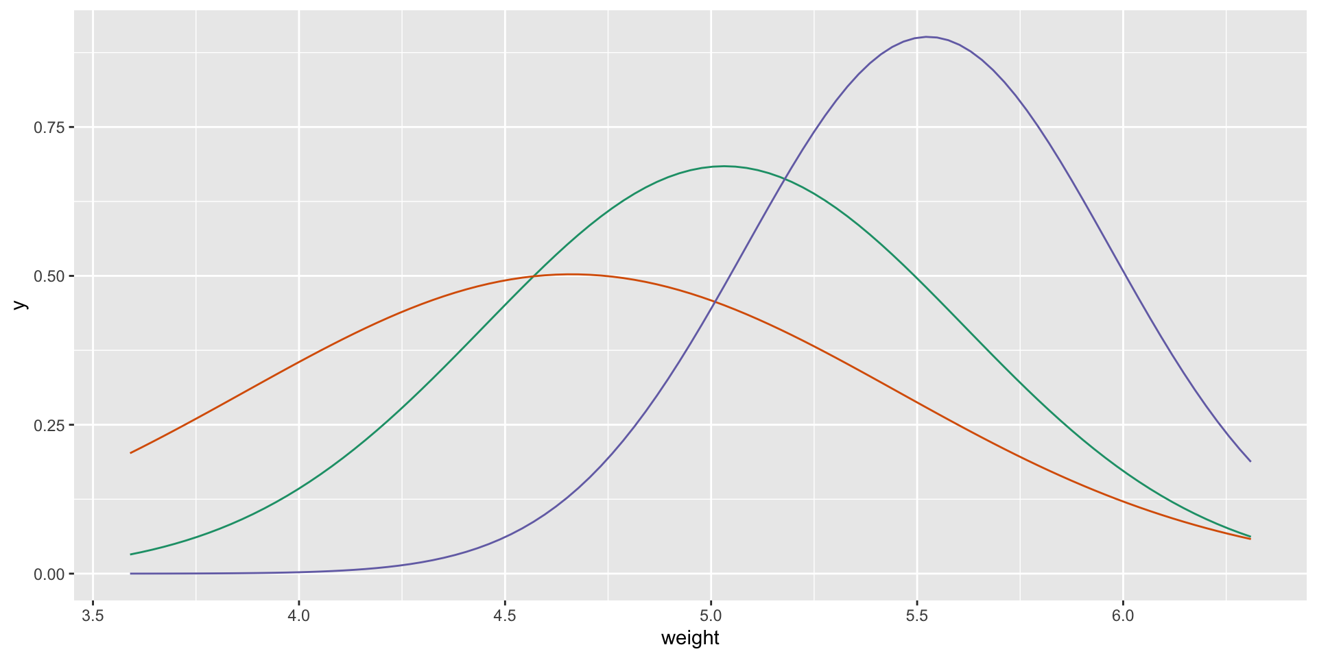
t-tests
t-tests assume that datasets are Normal distributions 1
The only input the test gets:
- mean \(\mu\), standard deviation \(\sigma\) for each group
Comparing multiple groups
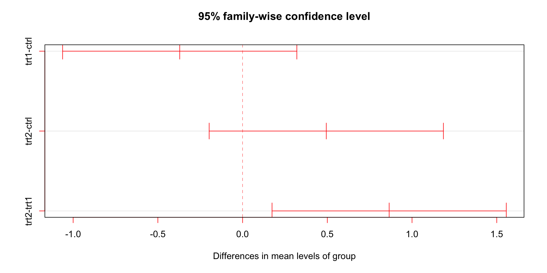
ANOVA allows blocking
This is important when using both sexes
But also if there are other batch effects to account for

Figure 3: MRC require that both sexes are used in experiments, unless there is strong justification not to.
ANOVA supports blocking

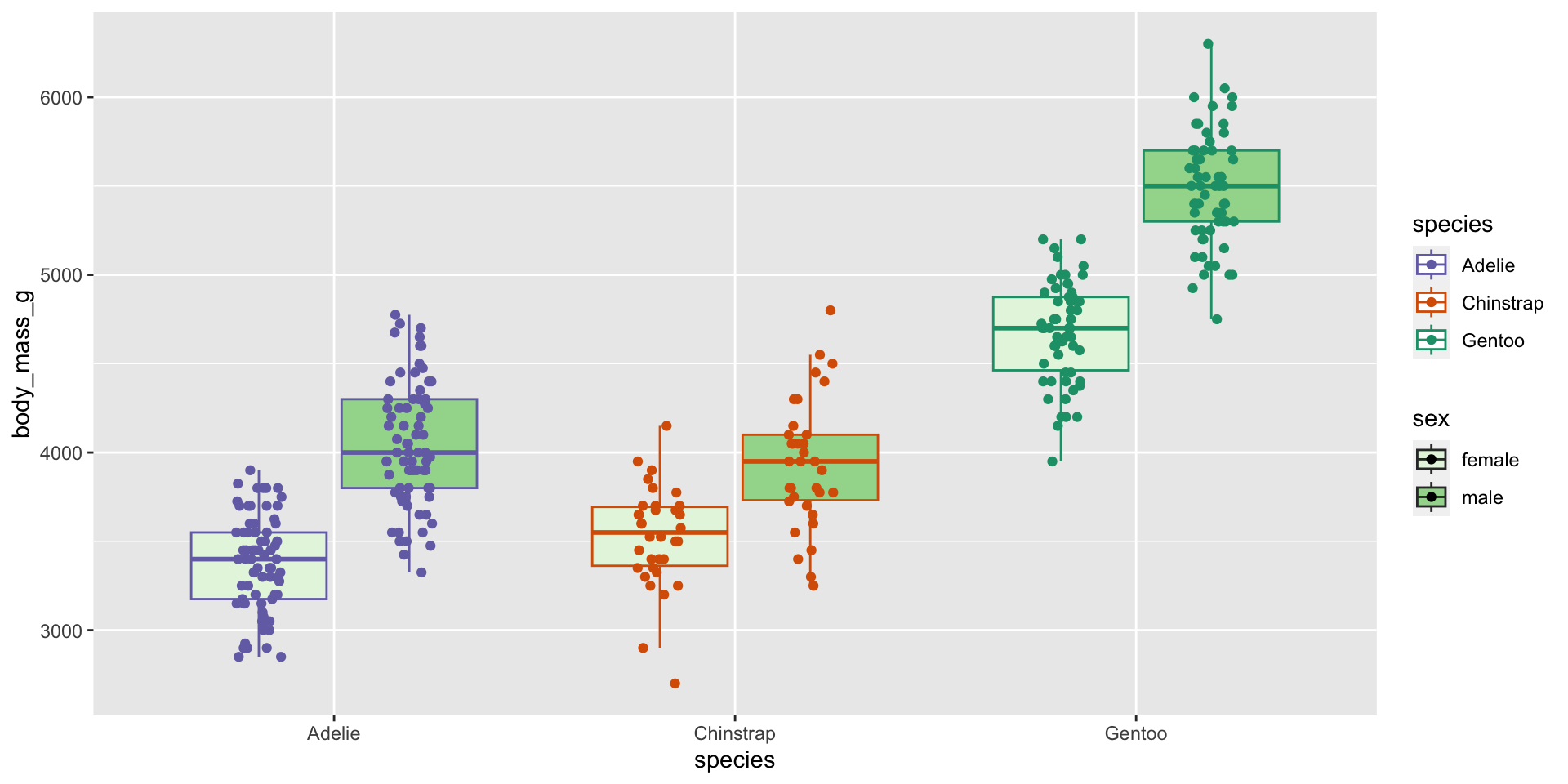
Visualise the dataset
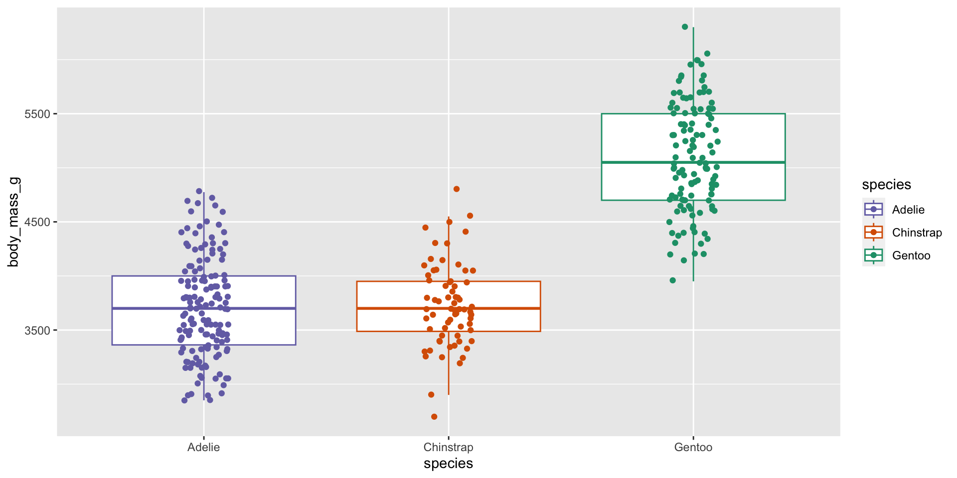
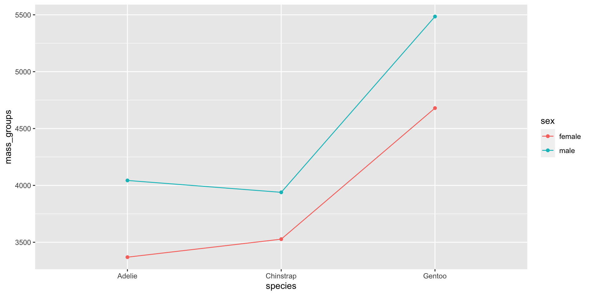
Visualise the dataset (sex differences)
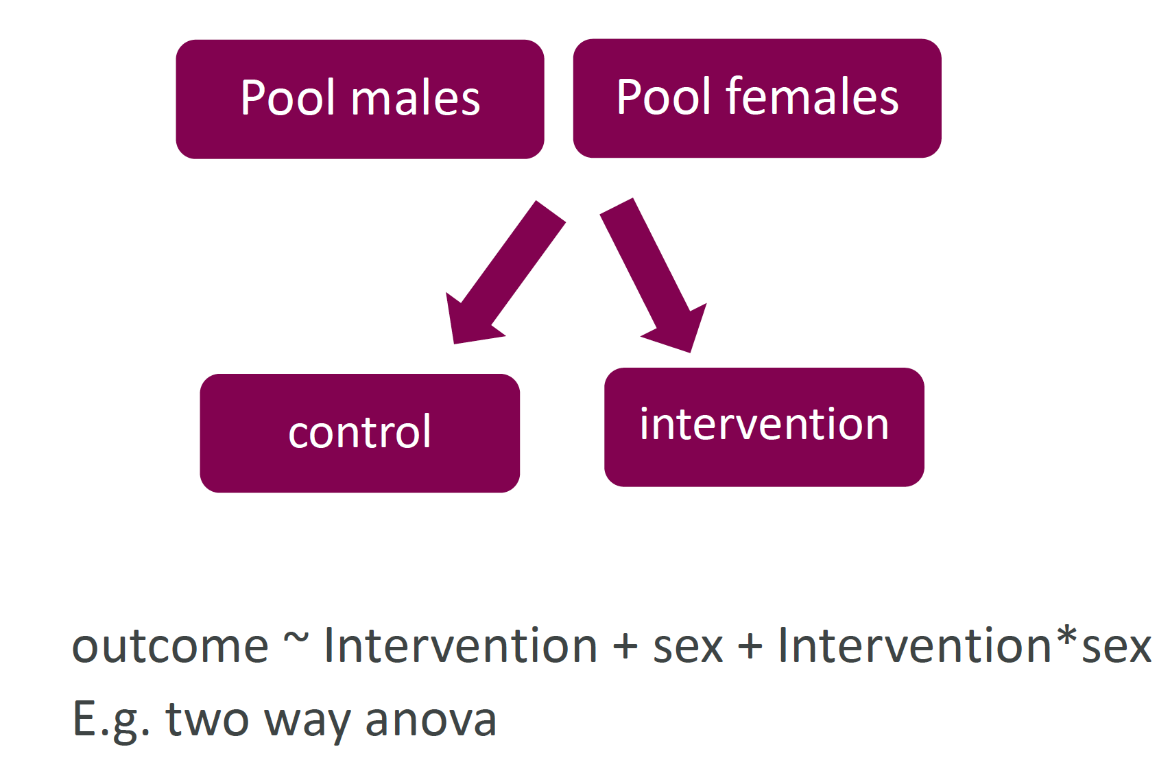
Interactions between categories
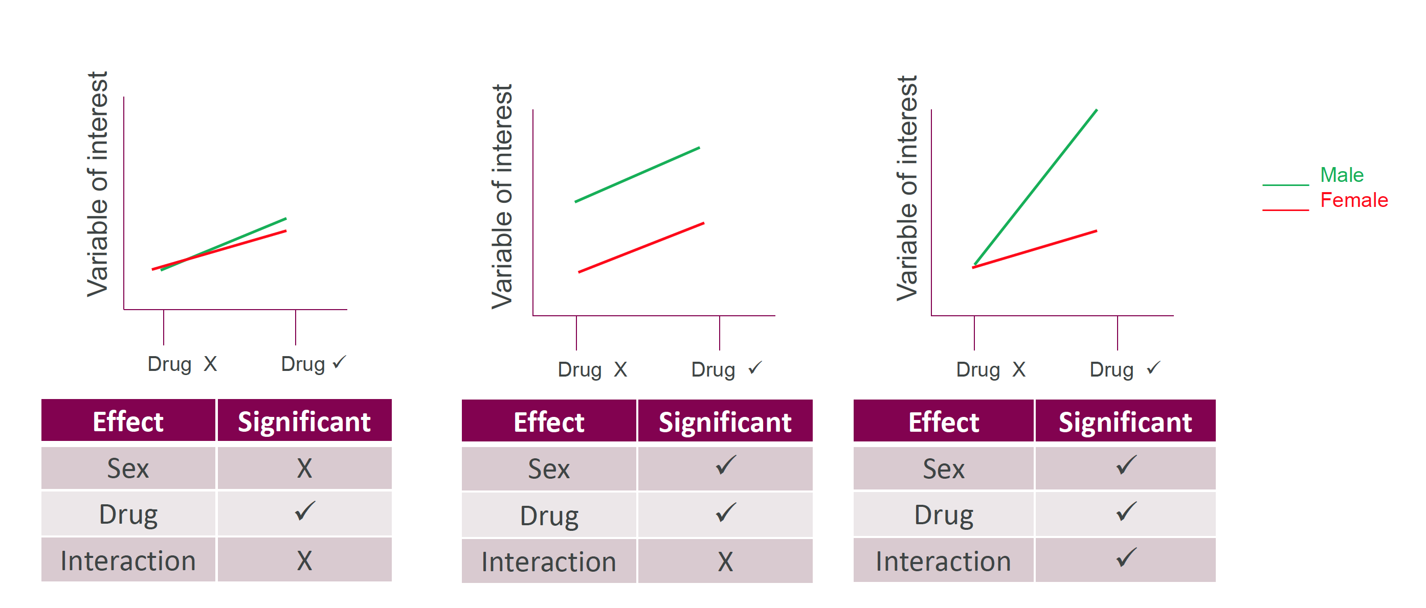
Figure 6: Two-way ANOVA lets us see interactions between categories
Interactions between categories
EDA may recommend ANOVA
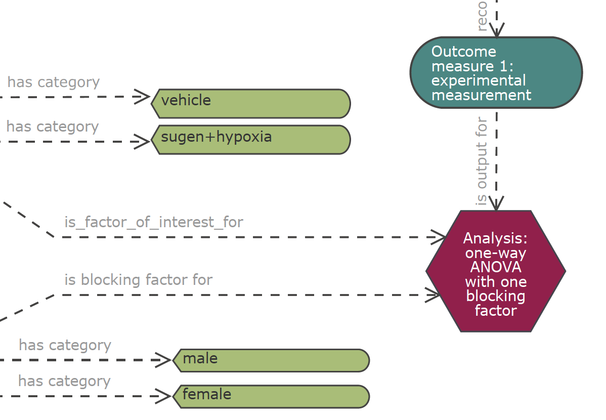
Figure 7: EDA may well recommend ANOVA
But NC3Rs EDA power calculations only cover pairwise t-tests!
G*Power
- Free software
- HHU Düsseldorf
- Windows and macOS
- Detailed manual
Supports ANOVA power calculation
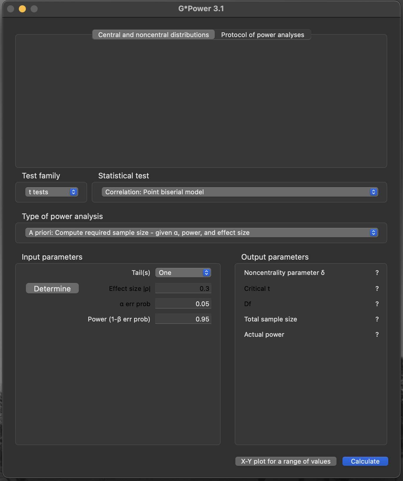
G*Power on macOSAn example
- Test family:
F tests - Type of power analysis:
A priori: Compute required sample size - given\(\alpha\), power, and effect size - Effect size \(f\):
0.4 - Error probability \(\alpha\):
0.05 - Power (\(1 − \beta\) error probability):
0.8 - Numerator d.f.: (2 − 1) × (2 − 1) =
1 - Number of groups:
4
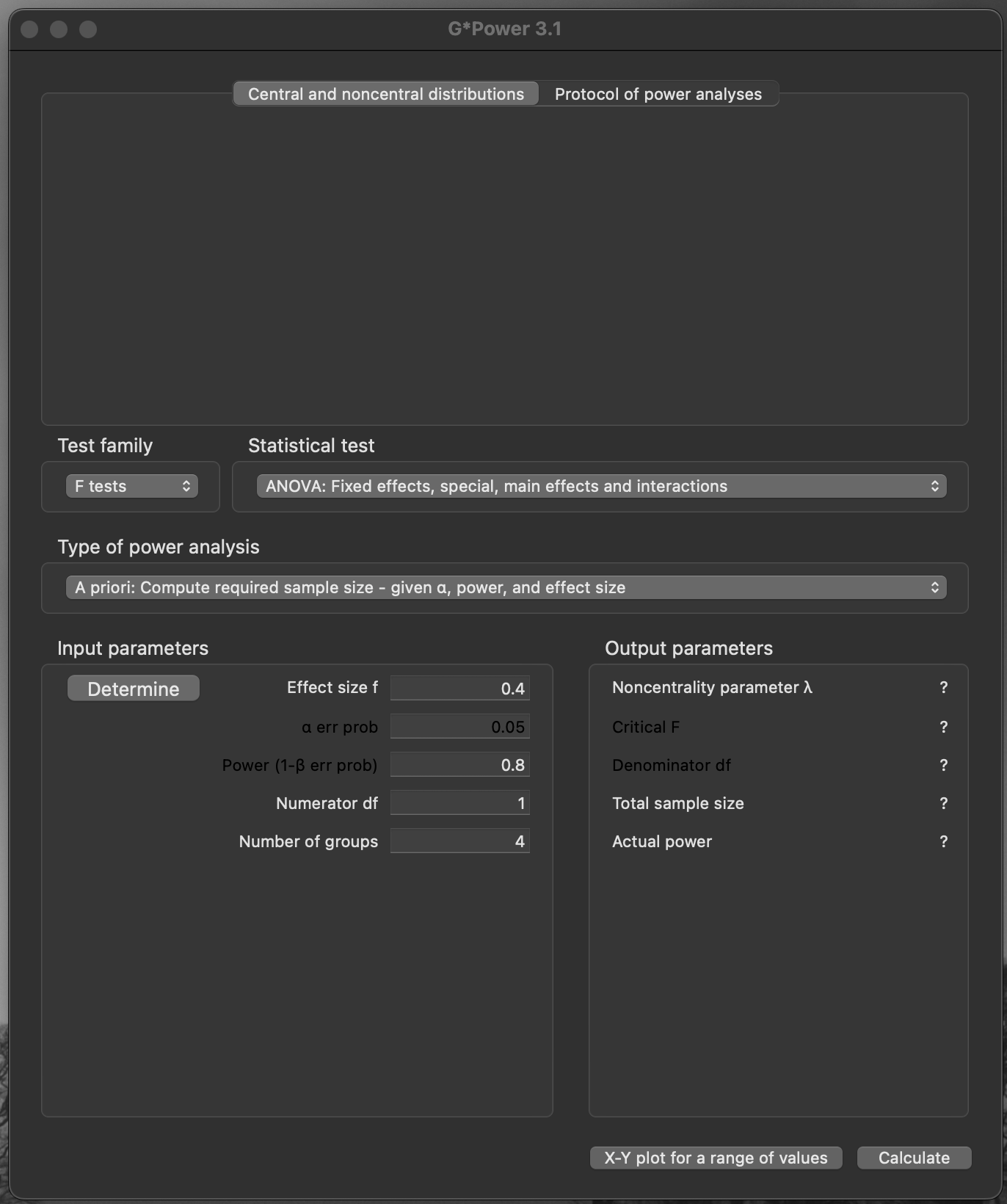
G*powerAn example
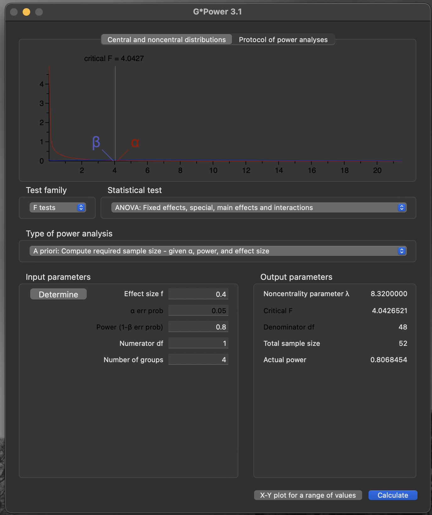
G*power outputAn example
G*Powerwill let you plot how sample size trends with desired power
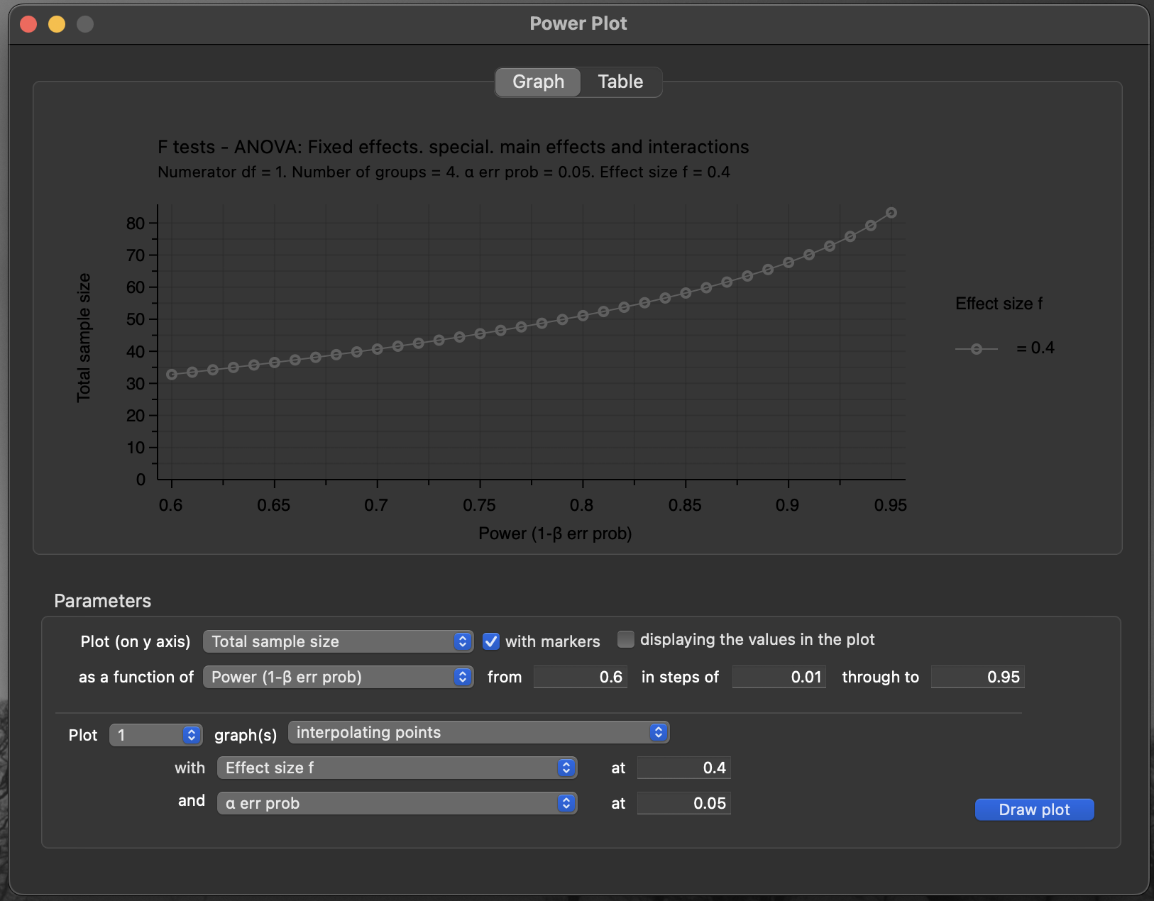
Figure 11: G*Power sample size vs power plot
An example
- The same plot with better colour choices (PDF output)
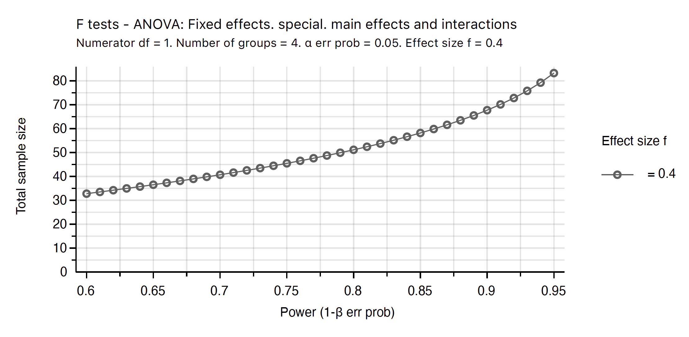
Figure 12: G*Power sample size vs power plot
Conclusions
Use NC3Rs EDA to formalise your design
Use ANOVA (where appropriate)
If using ANOVA, G*Power can calculate required samples for desired power