1  Introduction

This workshop introduces and reinforces concepts related to transmission and evolution of respiratory viruses.

1.1 Dendrograms (Tree Diagrams) and Evolution

In this workshop, you will produce dendrograms: these are tree diagrams that can represent the process of evolution. You have already seen tree diagrams, like those in Figure 1.1, used on this course to represent the process of evolution.

Figure 1.1: Tree of Life obtained using ribosomal genes, showing the major Domains of life. Reproduced from Hug et al. (2016).

Typically, in evolutionary analyses, you will see that these trees are organised to show a progression through time. The leaves of the tree usually represent things that exist “now” or, at least, most recently (these are at the right hand side of Figure 1.1).

The dendrogram traces lines - branches - from the leaves, and these gradually meet up together, just as branches of a real tree do, as you progress from right to left in Figure 1.1. Eventually, they all meet up together at the oldest (left-most, in Figure 1.1) part of the tree, (called the root).

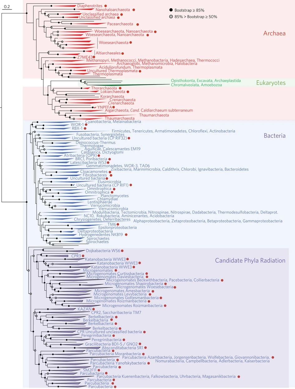
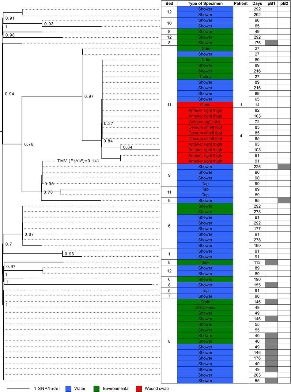
Trees like this can be used to represent large-scale evolution, like the complete Tree of Life in Figure 1.1, or evolution on a small scale. For example, Figure 1.2 represents evolution of the pathogenic bacterium Pseudomonas aeruginosa in a UK hospital. This tree was used to trace the source of infection in a burns unit, ultimately locating the precise valve in the plumbing from which the infectious agent was finding its way into patients (Quick et al. (2014)).

Figure 1.2: High-resolution genome-based phylogenetic tree of Pseudomonas aeruginosa samples collected during an observational hospital study to track infection. Samples were collected from wounds (red), water (blue), or the environment (green). All wound samples are closely-related to water samples from the shower next to bed 11. Reproduced from Quick et al. (2014)

1.2 Interpreting a tree

The trees in Figure 1.1 and Figure 1.2 both imply a branching evolutionary process. A single common ancestor to every organism represented at one of the leaves existed at some point in history, and that date in history is on the very leftmost point of the tree. The rest of the tree is a representation of how evolution progressed from that single ancestor to the variety of organisms represented at the leaf nodes.

1.2.1 Branch lengths

As you move from left-to-right in those trees, there is a short horizontal line (the root) that represents time passing for that ancestor. But then the branch splits into two (it diverges), representing some kind of event that produces distinct “offspring.” Each of these proceeds through time as a horizontal line for a distance before itself diverging to result in two new, differentiable offspring, and so on and so on until the leaf nodes are reached.

The lengths of the branches here represent, in some way, the passage of time between consecutive divergences (or a leaf node and the most recent split). The longer the branch, the longer the passage of time.

The length of a branch doesn’t necessarily correspond exactly to time

In practice, when we make these trees, we are usually measuring something other than time, itself. More often we are measuring some kind of difference between the leaf nodes, and assuming that a difference of 200 corresponds to 200 units of time (years, millennia, etc.), and a difference of 1000 corresponds to 1000 units.

Biology is complicated, and this assumption rarely holds exactly. There are methods to try to turn our measurements accurately into units of time, but they are beyond the scope of this course.

1.2.2 Cladograms and Phylograms

There is more than one kind of dendrogram. Two types you will meet frequently are:

• phylograms: each branch length is intended to represent the passage of time (or some other measure of difference) - they represent change on an evolutionary timescale
• cladograms: all branch lengths are the same - they do not represent change on an evolutionary timescale, only the order of divergences in the tree

(a) Phylogram.

(b) Cladogram

Figure 1.3: The same evolutionary tree represented as a phylogram, and as a cladogram. In a phylogram the branch lengths may be uneven. They represent evolutionary time between nodes (divergences and/or leaves on the tree), and the time between those may vary. In a cladogram the branch lengths are identical and the tree only represents topology - the order in which branches diverge.

1.2.3 Topology

Topology is the order of branching in a tree: the order of divergence events from the common ancestor of all leaf nodes to the present. Two trees with the same order of branching, but different branch lengths, have the same topology, and imply the same sequence of divergences.

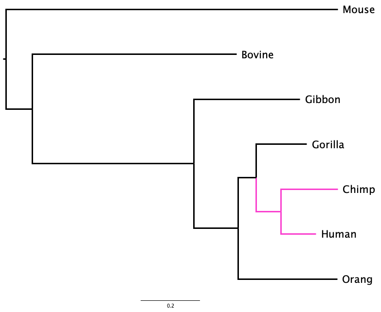
For example, in Figure 1.3 the first divergence separates Mouse from all the other mammals, and then the next divergence separates Bovine from the primates. Whether you examine the phylogram or the cladogram, the order of branching - the topology - of the tree is the same. They represent the same evolutionary sequence of events.

Note

Even if two trees share the same topology, and the same sequence of events, if any branch lengths differ the trees might still represent different evolutionary histories as the times between those events may differ.

Two trees can look superficially different, but actually represent the same sequence of branching events, and even the same evolutionary history, as is the case in Figure 1.4. Here, the tree has been rotated around the node that joins Human to Chimp. Although Human is above Chimp in one tree and below it in the other, both trees have identical topology.

(a) Original tree

(b) Tree with rotation

Figure 1.4: In any tree, branches can be rotated around an internal node without changing the structure or interpretation of the tree. Here, the two leaf nodes highlighted in purple (Figure 1.4 (a)) are rotated around their common ancestor to give the tree in Figure 1.4 (b). The rotated conformation is highlighted in green. Even though the two trees look different, the evolutionary relationships they represent are identical.

Question

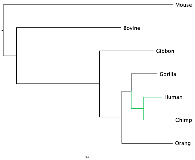
Is the tree represented in Figure 1.4 equivalent to the tree shown in Figure 1.3 (a)?

1.3 Evolution and Clustering

The examples in Figure 1.1, Figure 1.2, and Figure 1.4 are representations of evolution. In all cases, two organisms that share a more recent common ancestor (like Chimp and Human in Figure 1.4) combine together at a closer node than do two more distantly-related organisms (like Chimp and Gibbon).

It is natural to think of this representation as the divergence of species, as Gibbon diverging from ancestral primates at an earlier stage than Gorilla diverging from the ancestor of Chimp and Human. But it is also a representation of clustering. What this means is that we cluster Chimp more closely with Human than with Bovine because Chimp and Human share more similarities with each other than either do with Bovine.

In practice this means we can use mathematical approaches that cluster similar things together into trees to approximate evolutionary history, so long as what we use to measure similarity is relevant to evolution. Methods that perform this kind of clustering to produce a tree are called hierarchical clustering methods and you will use one of these to infer an evolutionary history for the `flu viruses you are evolving in the workshop.

Two different ways to reconstruct evolution

Hierarchical clustering methods are only one way to build an evolutionary tree. They were the first to be used, because they are not difficult to understand, and are relatively straightforward and quick to calculate. All of these methods apply an algorithm to construct a tree (or hierarchy - hence “hierarchical”) from a matrix (table) of distances between organisms. Methods that use this approach include Neighbour-Joining (Gascuel and Steel (2006)), and UPGMA. For these methods to produce an evolutionary tree, the distance we measure between organisms should reflect their evolutionary separation.

The development of cheap, powerful computing enabled more advanced and more accurate mathematical methods of evolutionary reconstruction to be used routinely. Such methods include Maximum Likelihood (ML, Xia (2018)) and Bayesian (Nascimento, Reis, and Yang (2017)) approaches. These methods require significant computing power and differ from hierarchical clustering because they attempt to fit statistically a model of evolution (like fitting a curve on a graph) to the data obtained from each organism, rather than using an algorithm to build a tree from distances.

In modern biology, a standard laptop can very quickly produce trees using Maximum Likelihood methods that fit an explicit and well-justified model of evolution. As a result algorithmic methods, such as Neighbour-Joining and UPGMA, which are prone to systematic errors and inaccuracies, and whose only real advantage was speed, are no longer considered good practice for evolutionary reconstruction.

If you’re interested in learning more about how we do this in practice, you might be interested in this course, by Dr Conor Meehan:

• Introduction to Phylogenetics

Let’s build a tree

Let’s get started with building a UPGMA tree by clicking on the link UPGMA (here, in the menu, or below)

Gascuel, Olivier, and Mike Steel. 2006. “Neighbor-Joining Revealed.” Mol. Biol. Evol. 23 (11): 1997–2000.

Hug, Laura A, Brett J Baker, Karthik Anantharaman, Christopher T Brown, Alexander J Probst, Cindy J Castelle, Cristina N Butterfield, et al. 2016. “A New View of the Tree of Life.” Nat. Microbiol. 1 (5).

Nascimento, Fabrı́cia F, Mario dos Reis, and Ziheng Yang. 2017. “A Biologist’s Guide to Bayesian Phylogenetic Analysis.” Nat. Ecol. Evol. 1 (10): 1446–54.

Quick, Joshua, Nicola Cumley, Christopher M Wearn, Marc Niebel, Chrystala Constantinidou, Chris M Thomas, Mark J Pallen, et al. 2014. “Seeking the Source of Pseudomonas Aeruginosa Infections in a Recently Opened Hospital: An Observational Study Using Whole-Genome Sequencing.” BMJ Open 4 (11): e006278.

Xia, Xuhua. 2018. “Maximum Likelihood in Molecular Phylogenetics.” In Bioinformatics and the Cell, 381–95. Cham: Springer International Publishing.