3 Types of Phylogenetic Tree
3.1 Introduction
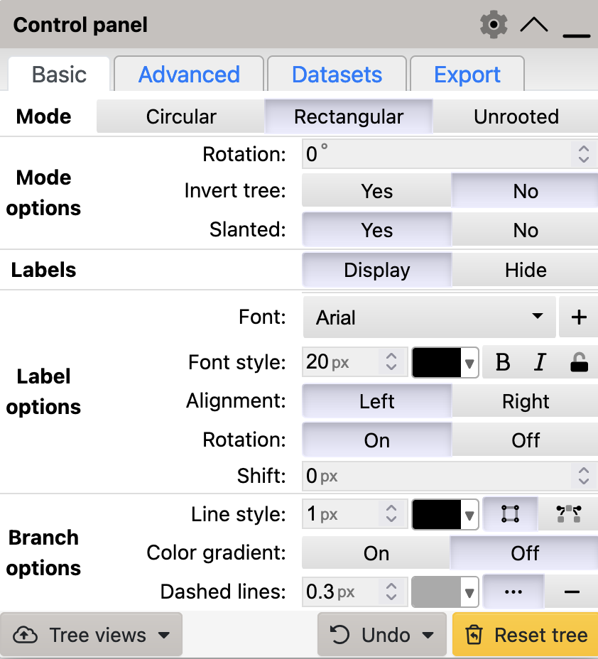
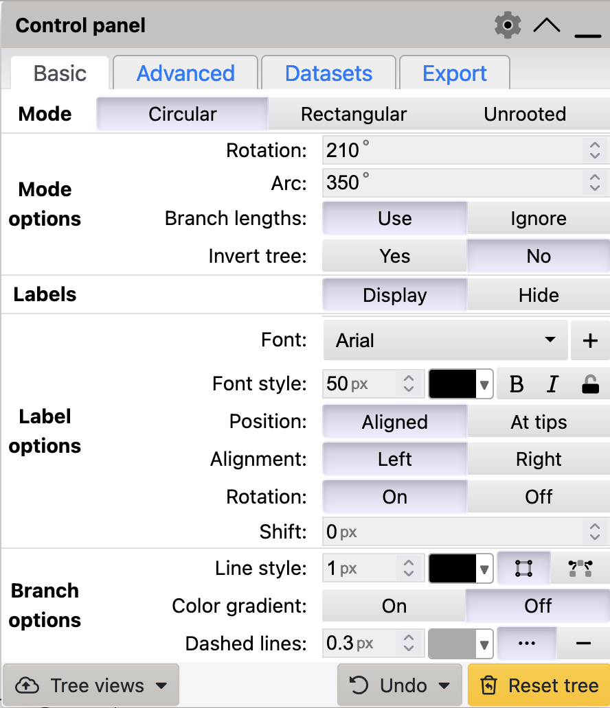
In this section, we will work through some of the visualisation options available in iToL to explore how the same phylogenetic tree can be presented to accentuate different aspects of the data. These options are managed through the control panel (Figure 3.1).
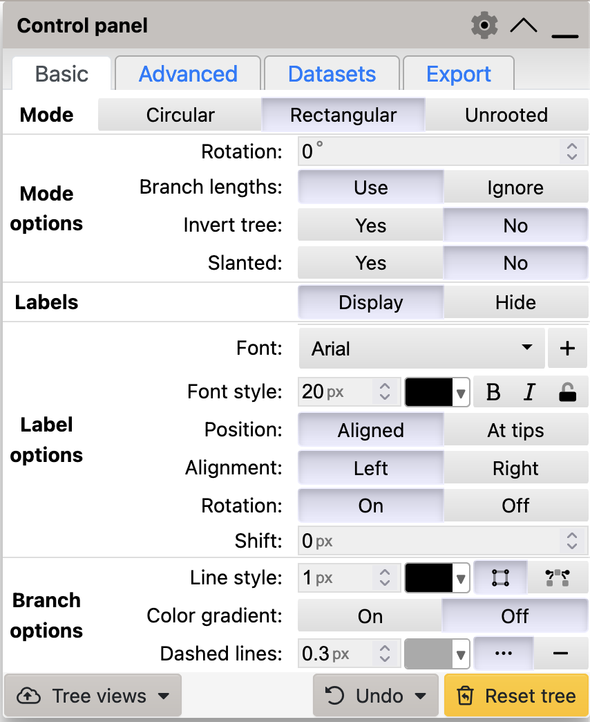
iTol control panel. Options in this menu allow you to change the way the tree is visualised.
3.2 Cladograms and Phylograms
The default tree presented by iToL (Figure 2.5) is a rectangular tree.
You can see from Figure 3.1 that the Rectangular mode is selected by default.
Broadly-speaking this means that the tree looks “rectangular” (it has lots of right angles) in a way that other tree representations do not. More specifically, every bifurcation is presented as a kind of “T-junction” where the ancestral lineage splits into two descendant lineages that leave the bifurcation at right angles (Figure 3.2)
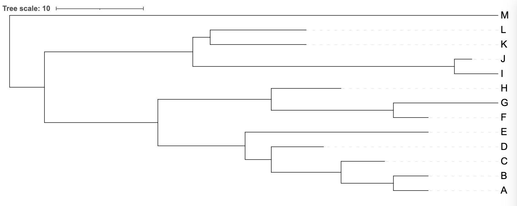
iToL view of the uploaded tree_newick.nwk tree is a rectangular tree - specifically a phylogram.
- a tree in which the branch lengths are proportional to the genetic change represented by the tree - this is called a phylogram
- a tree in which the branch lengths carry no meaning, or are an arbitrary length - this is called a cladogram
You can toggle between these two forms of rectangular tree in iTol by changing the Branch lengths: option from Use to Ignore (Figure 3.1). A cladogram shows the order of branching events, but does not provide visual information about the genetic change between nodes on the tree (branching events or leaves).
The order of branching events in a tree is referred to as its topology.

Branch lengths: option to ignore, iToL will show a rectangular cladogram.
3.3 Tree rotation
Rotating a tree does not change its content or the relationships it describes. All four trees in Figure 3.6 show exactly the same information. These trees were generated by setting the Rotation value in the iToL control panel (Figure 3.1).
iToL
To rotate your tree in iToL, use the Rotation setting in the Mode Options part of the Basic tab:
Basic tab has a Rotation setting that you can use to rotate your tree through any angle
Changing the scaling of the tree (stretching or compressing it in any direction) also does not change the information presented. The trees in Figure 3.6 were scaled horizontally by 50% using the Advanced tab of the iToL control panel (Figure 3.5).
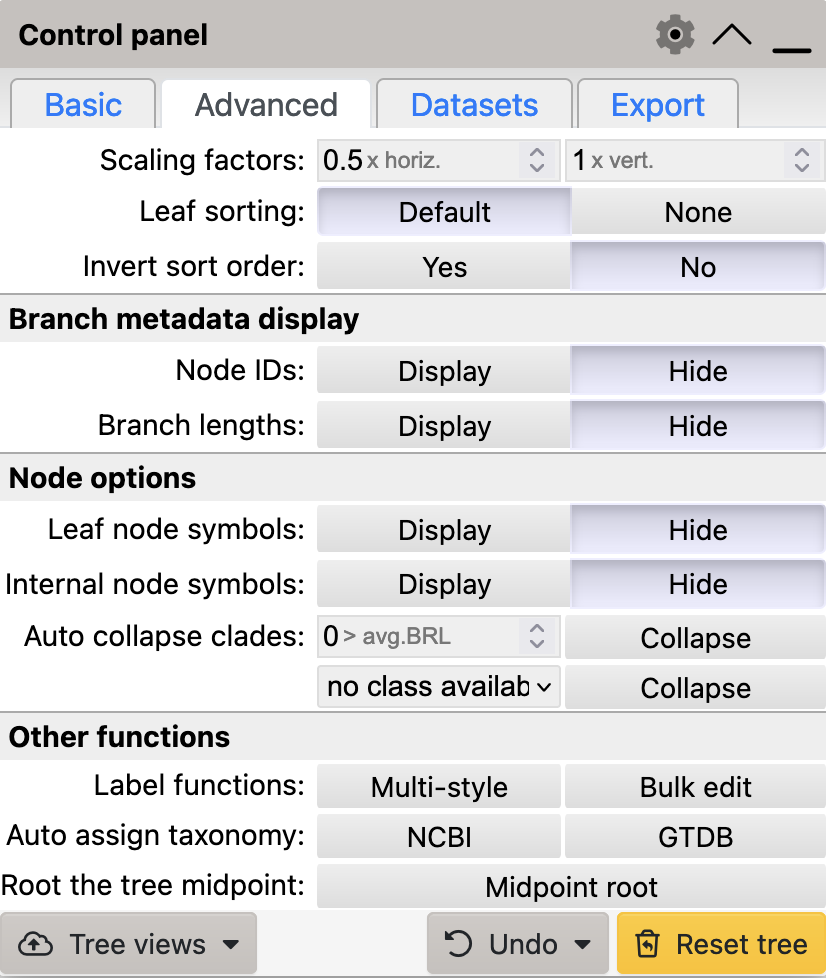
iTol control panel. Options in this menu allow you to change the way the tree is visualised.


3.4 Rotating clades
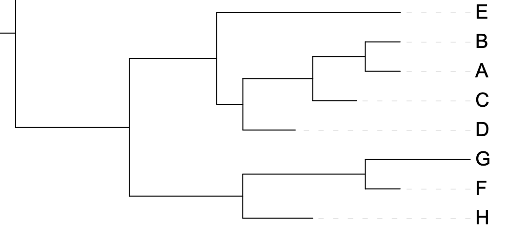
Rotating the members of a clade around their common ancestor also does not affect the content of the tree - and specifically leaves its topology (branching order) unchanged - even if it makes the tree appear visually quite different. The four trees in Figure 3.7 have exactly the same topology.
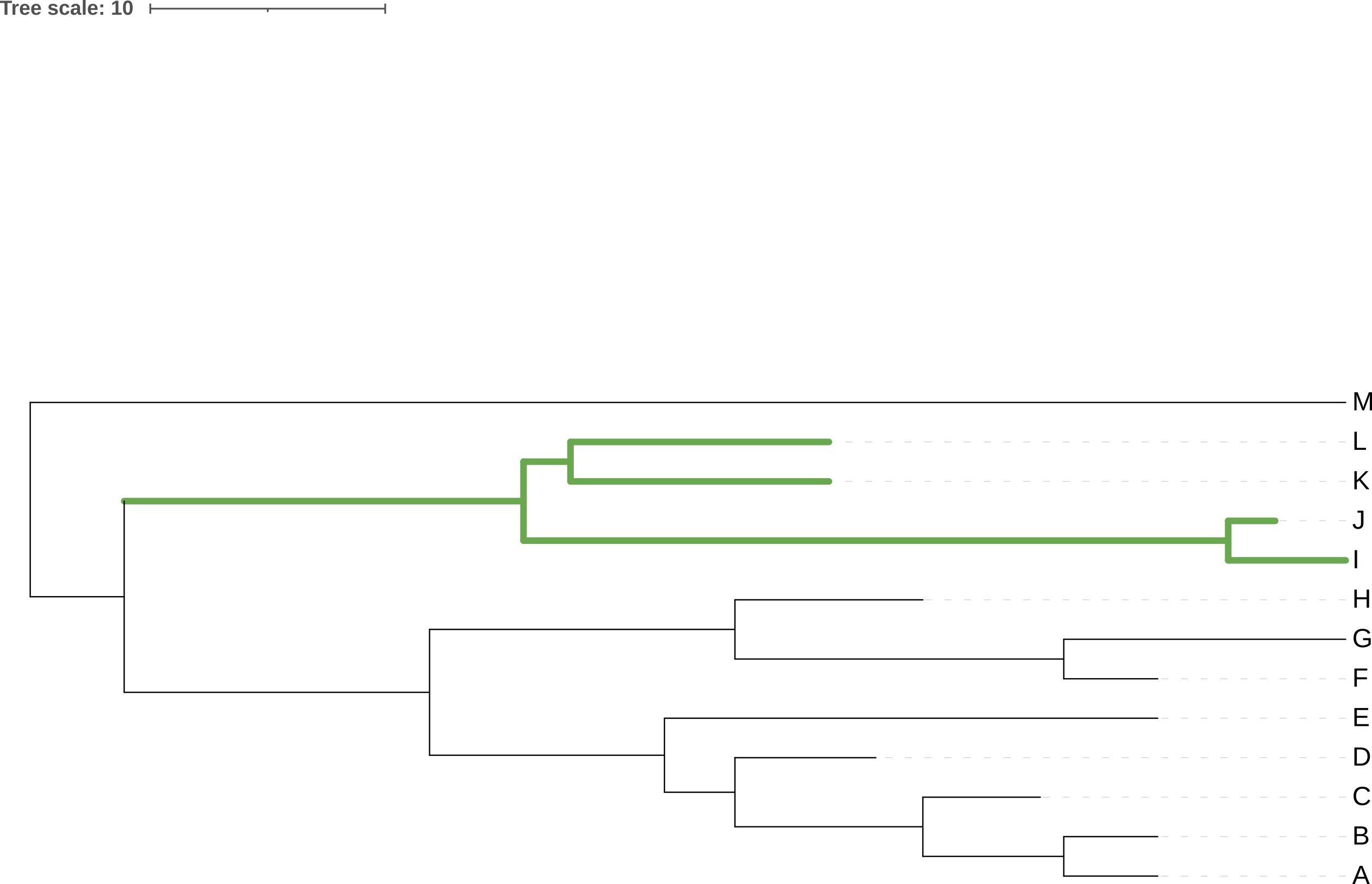
I, J, K, and L) highlighted.
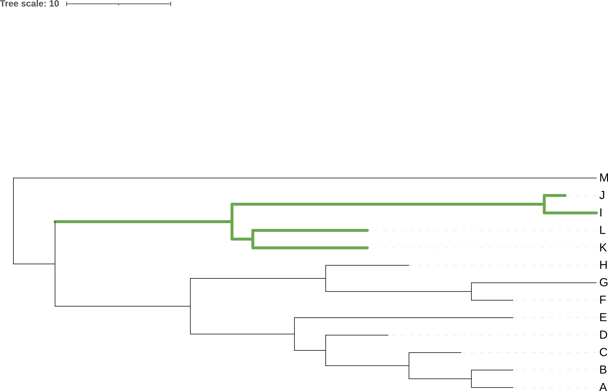
I, J, K, and L) around their common ancestor. This does not change the topology of the tree.
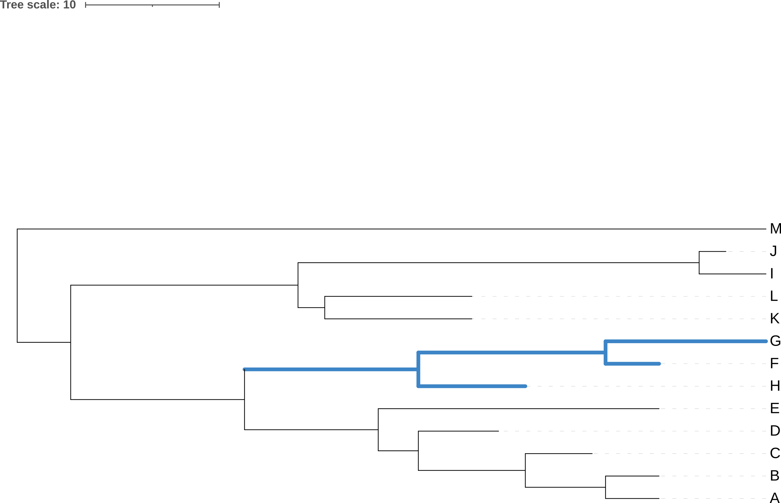
F, G, and H) around their common ancestor. This does not change the topology of the tree.
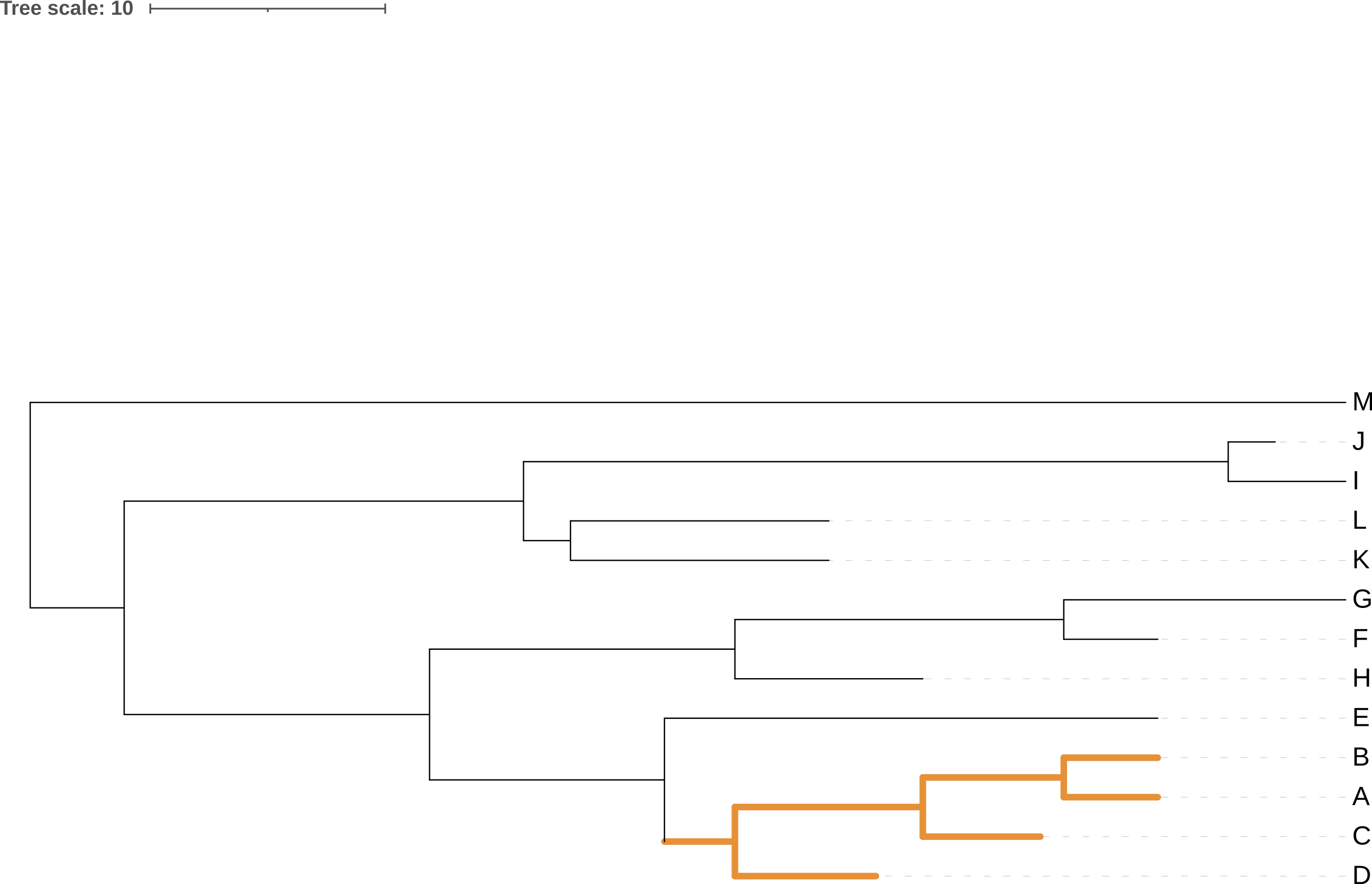
A, B, C, and D) around their common ancestor. This does not change the topology of the tree.
iToL
To rotate a clade in iTol, select the clade in the tree by clicking on its ancestral branch:
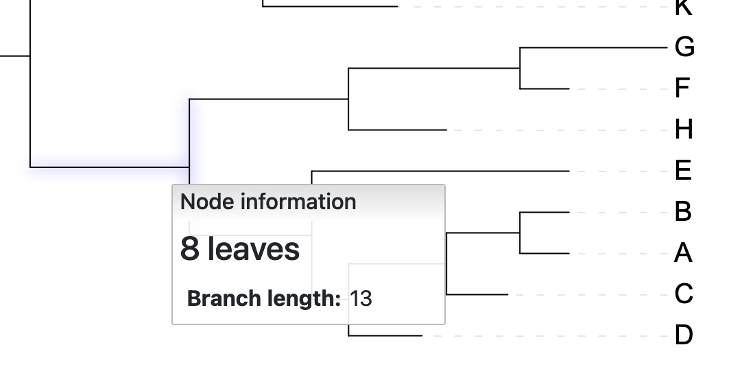
iTol by clicking on its ancestral branch
This will bring up a context menu that includes the action to Rotate children. Clicking on the Rotate children action will rotate the two “child” branches of the clade around their common ancestor.
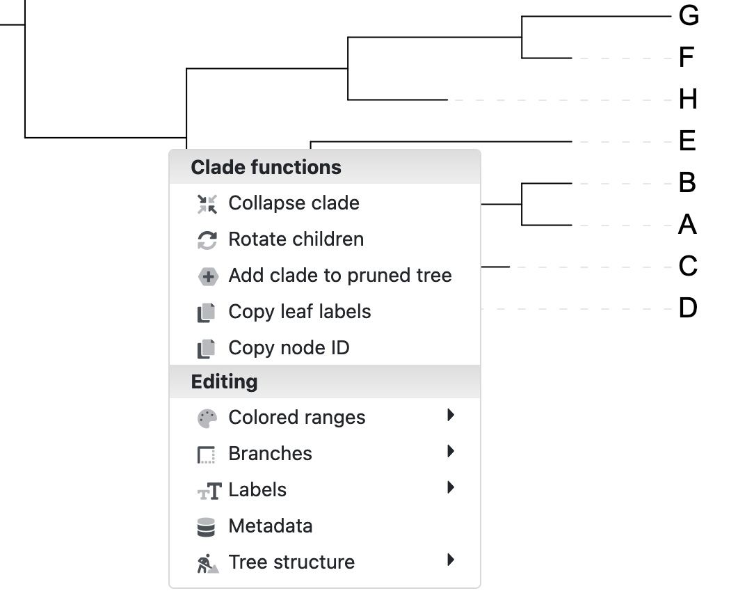
Rotate children action.
3.5 Non-rectangular trees
Phylogenetic trees do not need to be rectangular and, even if drawn using different forms, still present the same information as their rectangular counterparts.
3.5.1 Slanted cladogram
The angle formed at each branching event doesn’t need to be rectangular (at 90 degrees) - it can be narrower, as in a slanted cladogram. Figure 3.11 shows rectangular and slanted cladograms of the same tree. Being cladograms they provide only topology information, and this is the same in both renderings.


iToL
To generate a slanted cladogram in iTol, select Yes for the Slanted option in the Basic tab:
Basic tab has a Rotation setting that you can use to rotate your tree through any angle
3.5.2 Circular phylogram
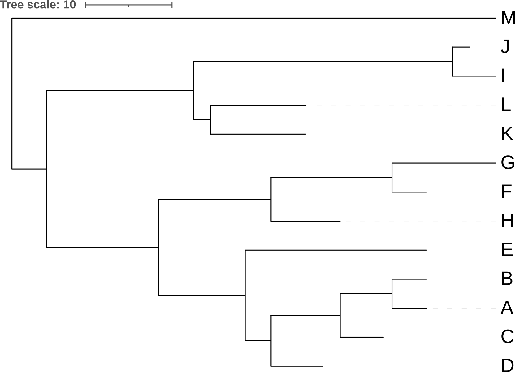
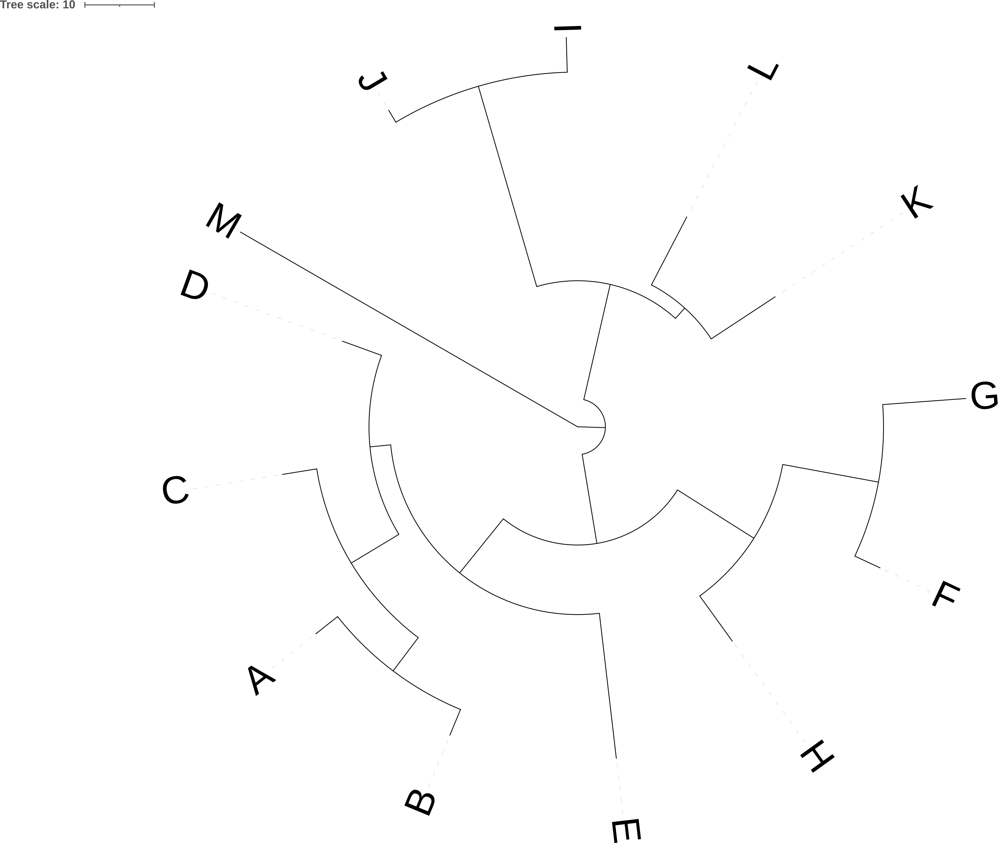
It is increasingly common, as datasets increase in size, to see circular phylograms in publications. These place the root at the centre of a circle and show the branches as radii with branching points moving away from the centre as genetic changes increase.
Rendering a tree in circular form does not change the information being presented, in comparison with a rectangular phylogram, as can be seen in Figure 3.13.
iToL
To generate a circular phylogram in iTol, select Circular mode in the Basic tab, and ensure that Branch lengths is set to Use:
Circular mode to generate a circular tree in iToL
Pros
- Circular trees use space on the page efficiently
- Circular trees are especially useful for fitting large trees into a small space, such as a journal page.
Cons
- It can be difficult to read the labels on circular trees easily
- Due to the way they are presented, especially for trees with lots of data, it can be difficult to see the branching order of nodes close to the root.
3.5.3 Unrooted trees
All the trees you have seen so far have an implied root - a single ancestral point from which all the sequences or species represented on the tree have descended. In terms of all life on Earth, we would call this root the Last Universal Common Ancestor (LUCA). For most trees we work with as scientists, the common ancestor would be much more recent than LUCA.
Some tree reconstruction methods, such as UPGMA or Neighbour-Joining (NJ) automatically produce rooted trees, because of the way their algorithms work.
Other, more accurate and precise, phylogenetic reconstruction methods such as Maximum Likelihood (ML) and Bayesian approaches (typically) produce unrooted trees. These methods do not (typically) produce a result that makes a claim about where the root of the tree is, so we often include an outgroup - a species/sequence, or set of species/sequences whose divergence point we already believe to be ancestral to the part of the tree we’re more focused on. This allows us to determine the most likely order of divergence in that part of the tree.
For example, if we wanted to produce a phylogenetic tree for primates, we would choose an outgroup such as lagomorphs (rabbits, hares, etc.) or colugos (Dermoptera), that diverged from an earlier common ancestor with primates (Perelman et al. (2011)).
Unrooted trees, like that in Figure 3.15, appear to extend out from a central point, but that central point may or may not be the real root of the tree. In Figure 3.15, the rectangular tree implies that the root, i.e. the point at which the last common ancestor diverged into the ancestor of M and the ancestor of the remaining species, lies somewhere between M and the last common ancestor of J and D, not at the central junction in the tree.

iToL
To generate an unrooted tree in iTol, select Unrooted mode in the Basic tab:
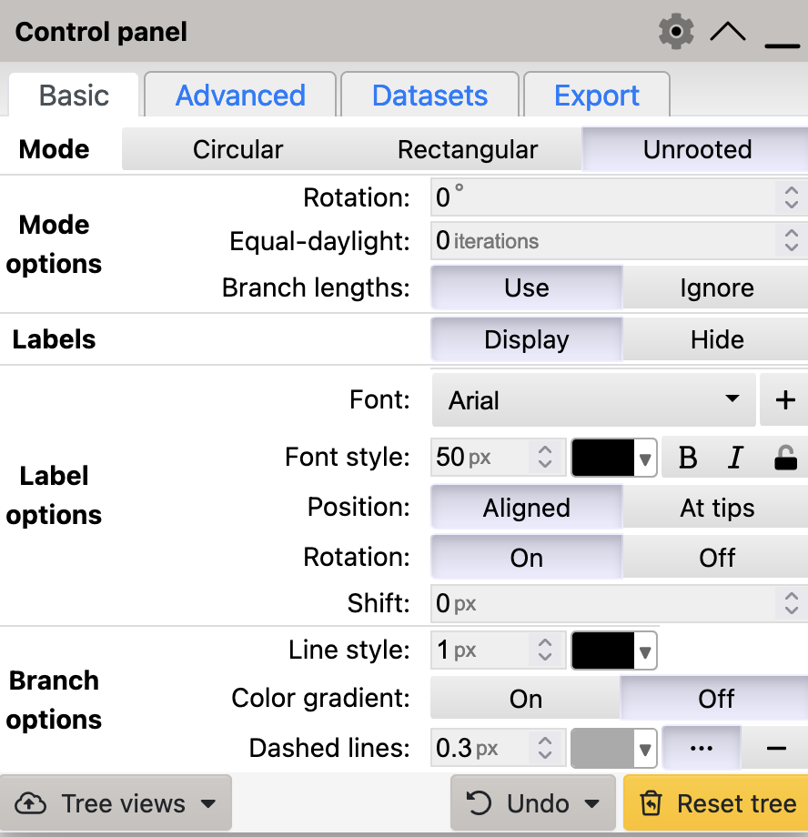
Circular mode to generate an unrooted tree in iToL
3.6 Summary
After successfully working through this section you should be able to:
- explain the difference between a phylogram and cladogram
- generate a rectangular phylogram and a rectangular cladogram using
iToL - describe and interpret the topology of a tree
- describe and interpret branch lengths of a tree
- explain how rotation of a tree, and clades within the tree, affects what the tree represents
- generate slanted cladograms, unrooted trees, and circular trees using
iToL
Please complete the workshop by answering the questions below in the formative quiz on MyPlace