5 Refining a Phylogenetic Tree Visualisation
5.1 Introduction
In Chapter 4 you used UniProt, MUSCLE, Simple Phylogeny and iTol to construct a tree from homologues of the BipC effector protein. The tree you generated will have resembled that in Figure 5.1, which is a reflection of the data, but is possibly not the most informative tree layout.

Simple Phylogeny, visualised in iToL.
In this section of the workshop, you will use iToL’s tools to make your tree more informative to a reader, using the tree you uploaded at the end of Chapter 4.
5.2 Re-rooting the tree
The Neighbour-Joining methodology that was used to build the tree in Simple Phylogeny assigns a root to the tree, although due to the way the algorithm works, this might not be the true phylogenetic root of the tree. We can inspect the tree without any assumption of root placement by examining the unrooted tree.
Use iToL to see the unrooted layout of your tree.
You should find what you need in Chapter 3.
Your unrooted tree should look something like that in Figure 5.2. There are two groups of sequences - one group closely related to each other (short branches) and one that is more diverse (longer branches).

Simple Phylogeny tree for BipC generated in iTol. There are two groups of sequences - one closely related (on the left), and one more distantly related (on the right)
The unrooted tree suggests that there might be two distinct groups of sequences, but this information looks to be masked in the default rectangular tree, so we will try re-rooting it for clarity.
A common approach to initial rooting of a tree, where an outgroup was not included in the analysis, is to use midpoint rooting. Midpoint rooting assumes that the root of the tree is halfway between the two most distantly-related sequences or species.
iTol
To use midpoint rooting in iTol
- Select the
Advancedtab from the control panel - Click on
Midpoint rootin theOther functionssection
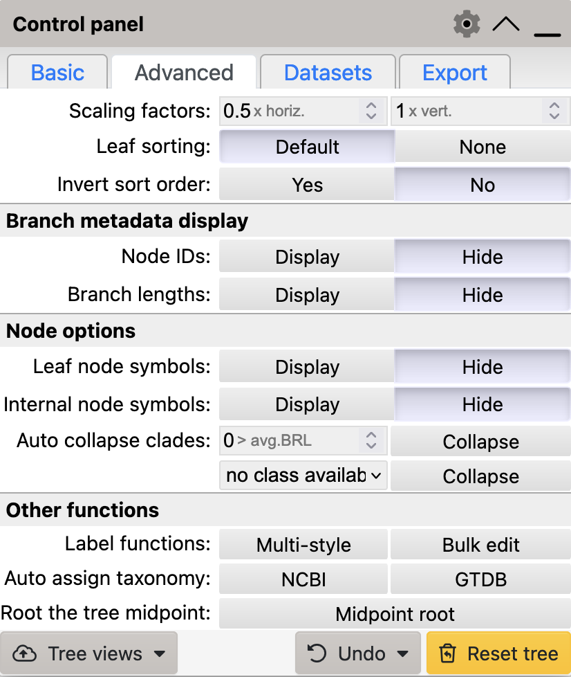
iTol’s advanced control panel tab
Use iToL’s Midpoint Rooting to modify the layout of your tree.
Your midpoint-rooted tree should look something like that in Figure 5.4 There is a group of recently-diverged sequences (sharing a recent common ancestor with short branches), and a group of more anciently-diverged sequences (sharing a recent common ancestor with longer branches).

Simple Phylogeny tree for BipC generated in iTol.
After midpoint rooting the tree, we might consider that there are two clades of interest - a recently-rooted clade, and a more anciently-rooted clade. It might be worth colouring these sequence groups in the figure, so we can refer a reader to them.
5.3 Highlighting clades
To highlight a clade in iToL by changing branch colour and thickness, first select the ancestral branch to a clade using your mouse, as in Figure 5.5.
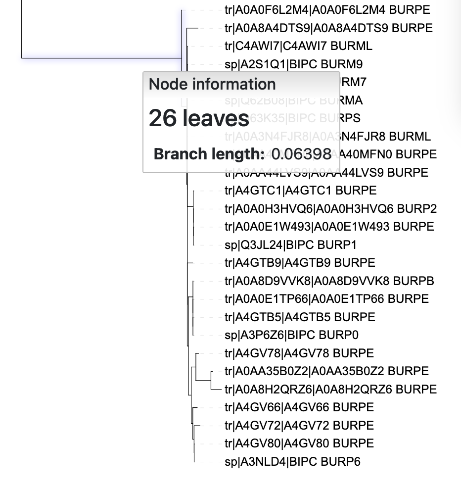
iTol tree.
Then bring up the context menu by clicking on the branch and select Branches -> Whole Clade to see colour and line thickness options (Figure 3.9). Set those options to whatever seems like a good visualisation choice for you.
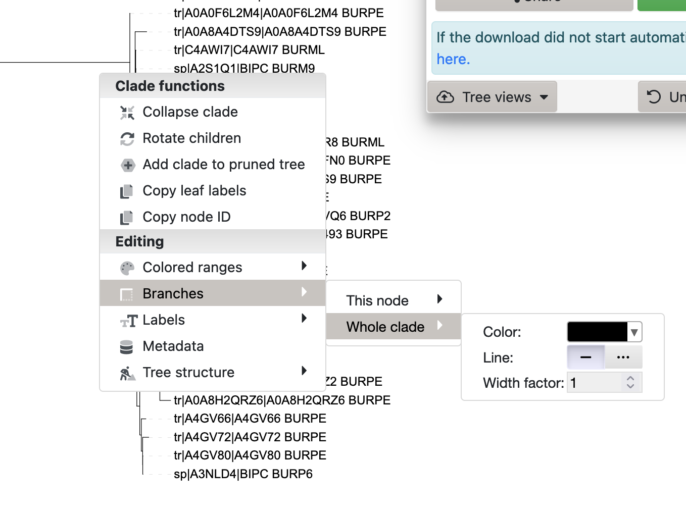
iToL context menu
Use iToL’s formatting options to highlight the more deeply-rooting clade in a way that distinguishes it from the more shallow clade.
The resulting formatted tree should look something like that in Figure 5.7.
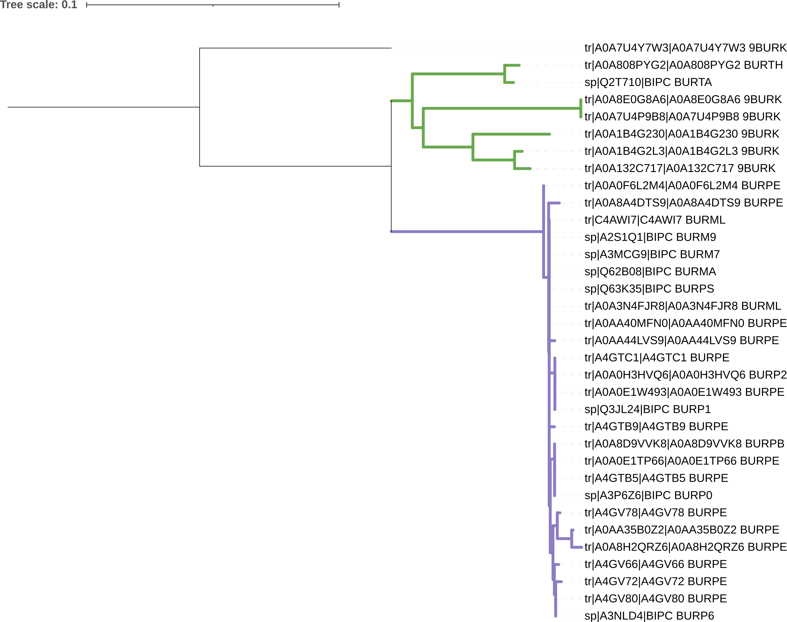
iToL.
5.4 Gene trees and species trees
Any phylogenetic tree we generate reflects only the data used to construct it. If we use sequences corresponding to a single gene or gene product, as we did for BipC, we generate a history only for that gene/gene product - this is called a gene tree.
We might assume that genes are transmitted vertically from parent to offspring but, in most life on Earth - i.e. microbial life, genes can also be transmitted horizontally and recombined into a different organism, maybe even a different species.
We cannot always assume that the history of a gene exactly represents the history of the organism it is currently found in.
As the history of any particular gene may not be the same as that of the organism it is found in, we have developed alternative approaches to construct species trees that are more reflective of the evolution of the species as a whole. These approaches are out of scope for this workshop, but include:
- whole-genome SNP trees
- multigene phylogenetic trees, essentially averaging over many single gene trees
- where a multigene tree includes every homologous gene across all the organisms involved, it is called a core gene phylogeny.
- whole-genome distance measures, like Average Nucleotide Identity (ANI) or digital DNA-DNA hybridisation (dDDH)
We would like to know how similar our BipC gene tree is to the known species tree for the organisms represented in it. We can tell which organisms are present in the tree by looking at the annotation label, specifically the final few characters:
9BURK: B. mayonis, B. humptydooensis, B. oklahomensis, Burkholderia sp.BURM7: B. malleiBURM9: B. malleiBURMA: B. malleiBURML: B. malleiBURP0: B. pseudomalleiBURP1: B. pseudomalleiBURP2: B. pseudomalleiBURPS: B. pseudomalleiBURP6: B. pseudomalleiBURPB: B. pseudomalleiBURPE: B. pseudomalleiBURTA: B. thailandensisBURTH: B. thailandensis
A core gene tree has been produced for this group of organisms - the B. pseudomallei complex (Hall et al. (2022)), and can be seen in Figure 5.8.
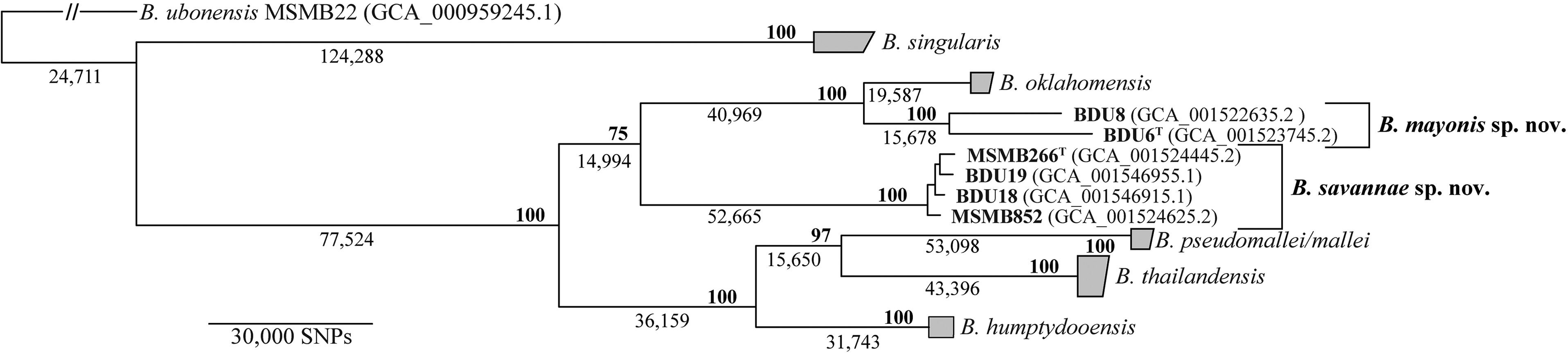
Compare the tree in Figure 5.8 to the tree you have produced from BipC.
- How are the trees similar?
- How do the trees differ?
B. mallei (glanders) and B. pseudomallei are the only pathogenic members of the B. pseudomallei complex (Janesomboon et al. (2021)). BipC is an effector protein that promotes infection of human and animal hosts.
- Considered in the context of the core genome tree in Figure 5.8, what does your tree suggest about the evolution of BipC?
5.5 Summary
After successfully working through this section you should be able to:
- midpoint root a tree in
iToL - colour highlight clades of a tree in
iToL - explain the difference between a gene tree and a species tree
- compare a gene tree with a species tree to interpret evolutionary history
Please complete the workshop by answering the questions below in the formative quiz on MyPlace