9 Visualise the Mapping
The .bam file generated in Chapter 8 contains the information we need to understand how well the reads map to a reference genome. However, being plain-text files and often quite large, they are not easy to read and process intuitively.
To get the most benefit out of these files, we usually visualise them using an appropriate software tool. The choice of tool depends on the reason for visualisation. The Artemis software (Carver et al. (2012)) is useful for interactive manual genome annotation; Tablet is an excellent tool for investigating genome assembly and sequence variation (Milne et al. (2013))1; and Proksee is an online service (Grant et al. (2023)) often used to obtain representative images of genome assembly annotations.
In this section, you will use JBrowse (Diesh et al. (2023)) to visualise your reference mapping interactively. JBrowse is a lightweight genome browser written in JavaScript that can run as a standalone application, or embedded as a web tool, as it is in Galaxy.
9.1 Visualising the Read Mapping
To use JBrowse to investigate your read mapping you need to tell it both what to display, and how to display it.
There are a number of new concepts being introduced here, and they may not make sense until you have tried to visualise your data.
If you follow the instructions below, and watch the video, you should find that everything works, and the meaning of unfamiliar terms like track group will become apparent.
- Navigate to the
JBrowsetool in theToolssidebar - Select the
JBrowsetool - Under
Reference genome to display, select theUse a genome from historyoption - Select the
GCF_000006765.1_ASM676v1_genomic.fnagenome file inSelect the reference genome - Click on
+ Insert Track Groupto add a new track group - In the new track group, enter
Mappinginto theTrack Categoryfield - Click on
+ Insert Annotation Trackto add a new track to hold the mapping data - Make sure that the
Track Typeof the new annotation track isBAM Pileups - In
BAM Track Data, select theBWA-MEM2.bamoutput file - Select
YesunderAutogenerate SNP Track - Click
Run Tool
JBrowse to visualise BWA-MEM2 mapping data
Click on the eye icon for the new JBrowse output. The magnifying glass icons can be used to zoom in and out of the visualisation. The check boxes to the left of the window can be used to control whether the reference genome and/or the annotation tracks are visible.
- Select the following tracks to be shown:
- Reference sequence
- Mapping (
SNPs/Coverage)
- Zoom in to the genome to obtain a visualisation of reads that map to the reference genome, similar to that in Figure 9.1.
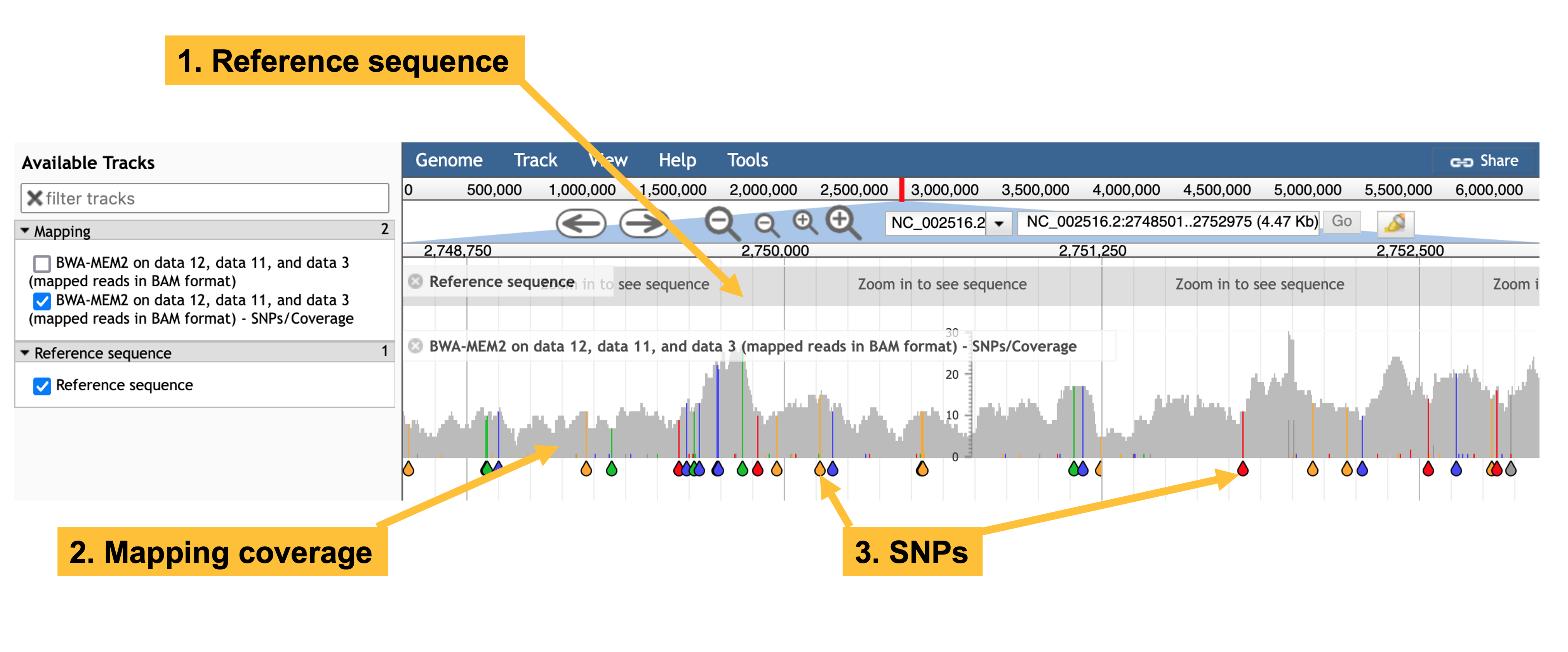
JBrowse visualisation of a BWA-MEM2 mapping ofERR531380 reads reads against a P. aeruginosa reference genome. The JBrowse tool shows the reference sequence (but zoomed out too far for individual bases to be visible), and a mapping track. The mapping track shows individual SNPs (teardrops), and total mapping read depth (the stacks above the teardrops).
You can click on the header of the SNP track in JBrowse and select Pin to top, so that you can zoom in and see individual SNPs, as in the video below.
JBrowse?
There is a short user guide on the JBrowse tool page in Galaxy. There is also official JBrowse documentation at the link below.
If you zoom out too far, you may not see any SNPs and may even see an error message reading Too many BAM features or Invalid array length.
If this happens to you, click on the Eye icon for the JBrowse output, and it should reset to the original view.
JBrowse
- Do the
ERR31380reads map uniformly to the same depth on the PAO1 reference genome? - When
ERR31380reads map to a SNP at the PAO1 reference genome, what proportion of the mapping reads contains the SNP, and what does that imply? - Based on the number of SNPs you can see in a 1,000bp region of the reference genome, estimate the total number on SNPs.
If the reads mapped uniformly, the grey plot of read depth would be flat and horizontal. It is not: there are many peaks and troughs. So the reads do not map uniformly - some parts of the genome are mapped more deeply than others.
By visual inspection, nearly all SNPs occur in all of the mapped reads. This implies that the SNP is a real sequence variant difference between the mapped and reference genomes.
Sampling a few 1,000 base regions I saw an average rate of about seven SNPs per 1kbp. The reference genome is around 7,000,000bp in length, so there are approximately 7,000 1kbp sections and I would expect around \(7,000 \times 7 \approx 49,000\) SNPs.
9.2 Next Steps
We can find SNPs by visual inspection in a tool like JBrowse, but there can be very many of them - as you can see. To ensure reproducibility and accuracy, and avoid errors we need to use dedicated software and pipelines when analysing mapping data. You will have a chance to do this in Chapter 10.
Tabletis the standalone tool I would prefer to use to visualise this data (LP).↩︎