10 Using G*Power
I hope by now you are convinced by the argument that a priori1 power analysis is an important part of designing experiments, and in the design of experiments where there are ethical considerations governing the numbers of experimental subjects, such as those using animals, in particular.
Unfortunately, power analysis is frequently overlooked by many scientists in their own experimental designs. The oversight is sometimes deliberate, and justified by arguments along the lines of “power analyses are too complex to perform”2 (Mayr et al. (2007)) Happily, there are widely-available software packages that make power calculations more accessible for all researchers.
In this chapter, we will walk through a calculation of power analysis using the widely-available and easy to use package G*Power(Faul et al. (2007)).
G*Power is a powerful software tool that can compute power calculations for a very wide range of statistical analyses, and several types of power calculation, including:
- a priori power calculation: conducted before the experiment is performed
- post-hoc power calculation: conducted after the experiment is performed - I would strongly discourage the use of post hoc power calculations.
- sensitivity: if the sample size is known, calculates for a given desired staistical power what effect size would be required to achieve that statistical power
It is beyond the scope of this workshop to consider all the possible circumstances that G*Power can accommodate, and our goal here is to introduce you to the basic functionality of the program.
10.1 Useful links
G*Powerhome page; downloadG*Powerfrom this siteG*Powermanual
10.2 G*Power Walkthrough: one-sample t-test
In this walkthrough we will consider a simple statistical analysis to determine whether the average weight of ten mice is statistically different from 25g.
10.2.1 Preliminary questions and assumptions
This is about as simple a case as we might want to consider, but we still need to answer some questions before we start:
- We know that mean values of samples from populations tend to follow a Normal distribution, so this suggests a t-test is appropriate.
- We are testing the mean of a sample against a single hypothesised central value, so this is a one-sample t-test.
- As we want to know if the sample mean is different from that single stated value, we require a two-tailed test.
- We want to determine an appropriate sample size for our experiment
- As we want to know a good sample size for our experiment, before the experiment is conducted, this is an a priori power calculation.
- We will use a standard funder’s requirements of 80% power at a \(P < 0.05\) threshold for statistical significance.
- i.e. \(\alpha = 0.05, \beta = 0.2, 1 - \beta = 0.8\)
- We will assume that a 10% difference in weight from the target 25g is meaningful, for an effect size of 2.5g.
- We will assume that the weight of individuals in the sample has a standard deviation of about 1.25g
- i.e. \(\sigma = 1.25\)
10.2.2 Walkthrough
- Open the
G*Powerapplication, to see the default settings (Figure 10.1).
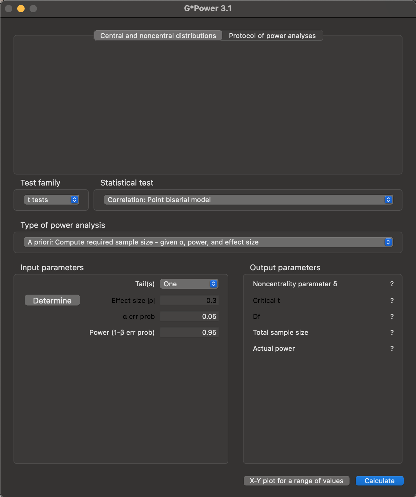
G*Power. This presents three panels: at the top is a space where output will be shown; in the middle, we can select the kind of statistical analysis we want to perform (Test family, Statistical test), and the kind of power analysis we’d like to carry out (Type of power analysis); below this is a set of fields where we can enter parameters for the power calculation, and where results will be displayed.
- Set the appropriate values for the statistical analysis we want to perform: one-sample, two-tailed t-test (Figure 10.2).

G*Power settings for our analysis. The Test family was already set to t tests, but we had to change (i) the Statistical test option to Means: Difference from constant (one sample case), (ii) Type of power analysis to A priori: Compute required sample size - given $\alpha$, power, and effect size, and Tail(s) to be Two.
- Set input parameters for statistical power and significance. We have chosen a statistical significance threshold of \(\alpha = 0.05\) and power as \(1 - \beta = 0.8\), and can enter these values directly (Figure 10.3).
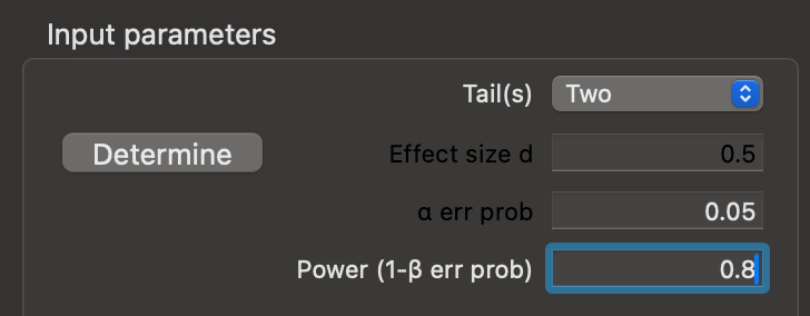
Input Parameters pane of G*Power with appropriate values set for statistical power and significance.
- We still have to enter the effect size in the
Input Parameters.G*Powerexpects something called Cohen’s d, not the absolute effect size of 2.5g - so we must calculate this. Click on theDeterminebutton to open the effect size drawer and enter appropriate values forMean H03,Mean H14, and$\sigma err prob5, then clickCalculate and transfer to main window(Figure 10.4).
Cohen’s d is an effect size index, which is a way of turning the expected means and variations from comparisons at very different quantitative scales into a single comparable value. To calculate d, we use the equation:
\(d = \frac{\mu - \mu_0}{\sigma}\)
where
- \(\mu\) is the mean of the null hypothesis
- \(\mu_0\) is the mean of the alternate hypothesis
- \(\sigma\) is the estimate fo the (unknown) standard deviation in the population
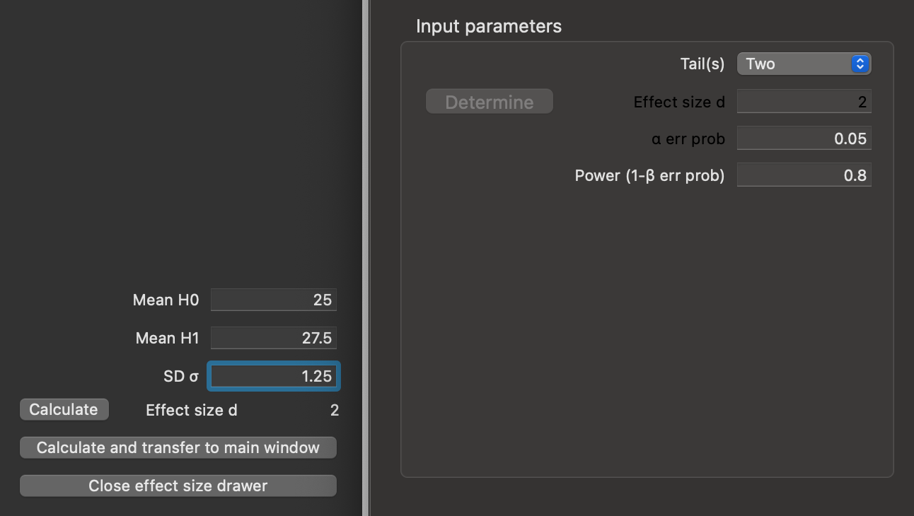
G*Power effect size window with our hypothesised mean values, and standard deviation, reporting a Cohen’s d for this comparison of 2. The Calculate and transfer to main window button has been pressed, which populates the Effect size d field of the Input parameters pane.
- Click the
Calculatebutton to obtain the results of the power calculation (Figure 10.5).
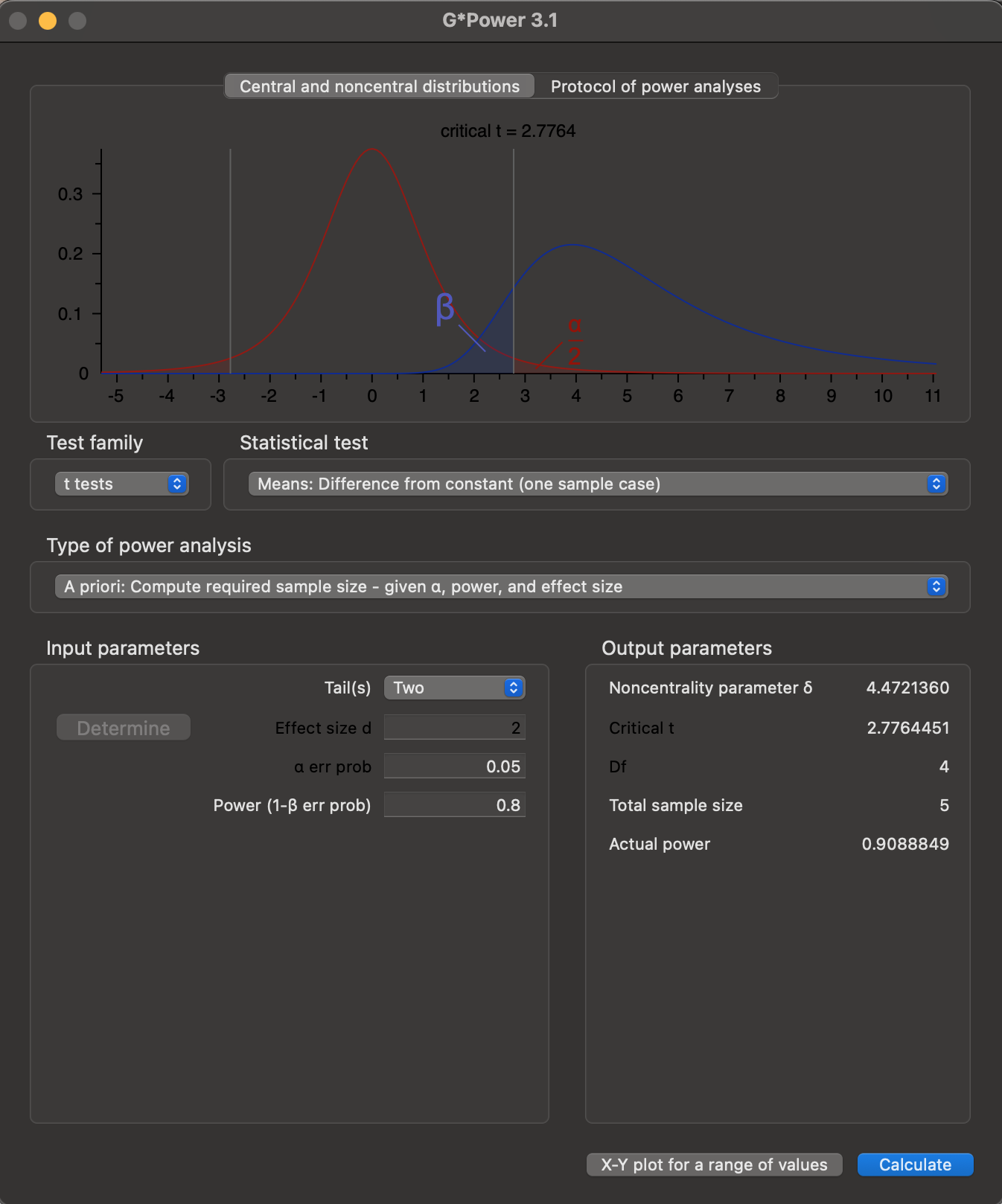
Output parameters pane, and a graphical representation of the likely statistical outcomes given the input parameters is shown in the topmost pane. Clicking on Protocol of power analyses provides a summary of the power calculation settings.
- Click on the
X-Y plot for a range of valuesbutton. This will bring up a newPower Plotwindow, automatically populated with the settings from our analysis (Figure 10.6).

Power Plot window, autopopulated with values from our power analysis.
- Click on the
Draw plotbutton to obtain a graph showing how required sample size varies with desired power, with our analysis settings (Figure 10.7).
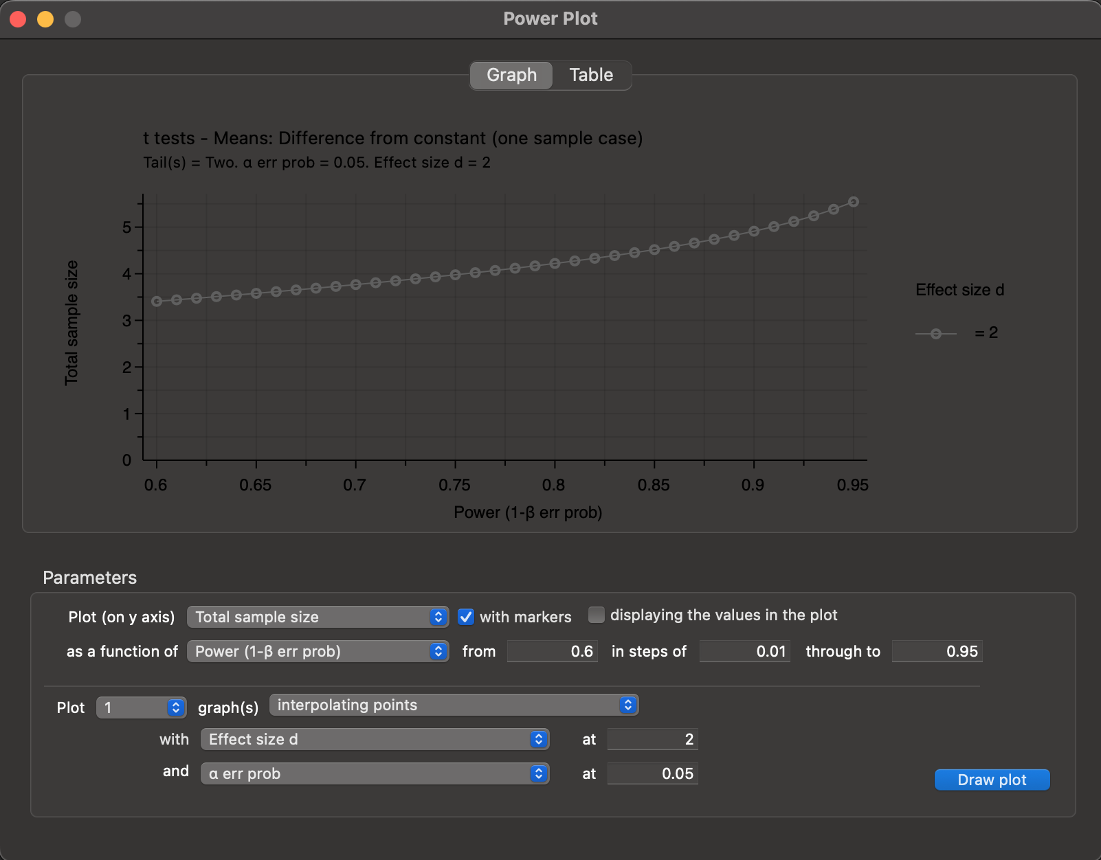
Power Plot window, showing how sample size varies with desired power, for our chosen settings.
- You can save the graph as a
.pdffile as shown below, by choosingFile -> Save x-y plotfrom the top menu (Figure 10.8).
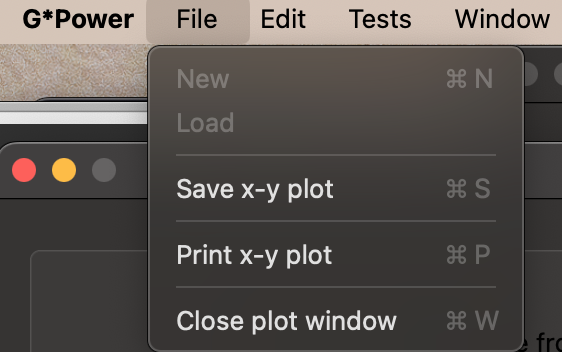
File -> Save x-y plot option to save the Power Plot graph.
10.2.3 Interpreting the output
The results indicate that we need a sample size of at least \(N = 5\) experimental units to ensure a power \(1 - \beta \geq 0.8\), with \(\alpha = 0.05\).
The actual power achieved with this sample size \(N = 5\) is \(1 - \beta = 0.9088849\), which is higher than that requested. We can use the Power Plot graph output to investigate how the predicted power of the experiment would change if we modified the sample size \(N\).
10.3 Manual and Tutorial
The current manual is found at this link.
This tutorial is published as Mayr et al. (2007).
Before the experiment takes place.↩︎
Although it could be noted that, if the power analysis is too complex for the researcher, we should be open to the possibility that the experiment is too complex for the researcher.↩︎
This is the null hypothesis - for us, the null hypothesis is that there is no difference between the mean of our sample and the constant value of 25g, so set this to be
25.↩︎This is the expected mean of the alternative hypothesis. Our assumed effect size of 2.5g implies that this expected mean is 27.5g.↩︎
This is the estimate of the standard deviation of the population. Our estimate is that this is 1.25g.↩︎