26 Modelling the Experiment
Before designing any experiment it is useful to think conceptually about what you know (or believe) about the way that the samples you will take and measure are produced by the system under study. This is primarily a scientific description of the experiment, not a statistical one.
Experimental design is the incorporation of the knowledge and expertise you have into a system that explains how the measured results are influenced by the experimental factors under your control1.
26.1 Variables in this experiment
Variables in an experiment include those things that you can observe and are expected to influence the measured outcomes of that experiment. These might be under your control (such as drug concentrations), or outside your control, but potentially influential (e.g. the sex of the subject, the technician working on that day, and so on).
Variables can also represent things that you cannot observe, but want to estimate. For our example experiment here that would be the proportion of the Earth’s surface that is water. But in a “real” experiment this might be “the effect of the administered drug on blood glucose concentration.” We can’t measure that directly, the same way we can’t measure the proportion of the globe’s surface that is water, but we can estimate it with our experiment.
Variables can be measured outcomes of an experiment. Here, our counts of the number of times our index fingers land on water (W) or land (L) are variables we will use in our estimate of the proportion of water on the Earth’s surface.
The variable we want to estimate is called the estimand. Here it is the proportion of the Earth’s surface that is water, but it might be something like “the reduction in blood glucose concentration” in a “real” experiment.
Variables under the experimenter’s control, where we want to investigate the effect of the variable on the estimand are called independent variables.
Variables whose values are expected to change when we modify an independent variable are called dependent variables.
Variables that may affect the dependent variables, but which we are not investigating directly are called nuisance variables. We may need to control for the influence of these variables, in our experimental design.
26.1.1 \(p\): The proportion of the Earth’s surface that is water - our estimand
The thing we want to estimate, our estimand, is a variable representing the proportion of the globe that is covered with water. We’ll assign this the letter \(p\) (for proportion). We cannot directly observe this value2. We can only measure it indirectly.
26.1.2 \(W\): The number of times our index finger lands on water - a measured outcome
This is the count of the number of times our index finger lands on water. We are observing this directly and assign it the letter \(W\) (for water).
26.1.3 \(L\): The number of times our index finger lands on land - a measured outcome
This is the count of the number of times our index finger lands on land. We are observing this directly and assign it the letter \(L\) (for land).
26.1.4 \(N\): The total number of times we toss the globe - an independent variable
The number of times we throw the globe and make a measurement is entirely under our control, and influences the measured outcomes of the experiment. The more times we toss the globe, the larger we expect \(W\) and \(L\) to get. We assign this variable the letter \(N\) (for number), and it is the independent variable in our experiment.
26.2 How do variables influence one another?
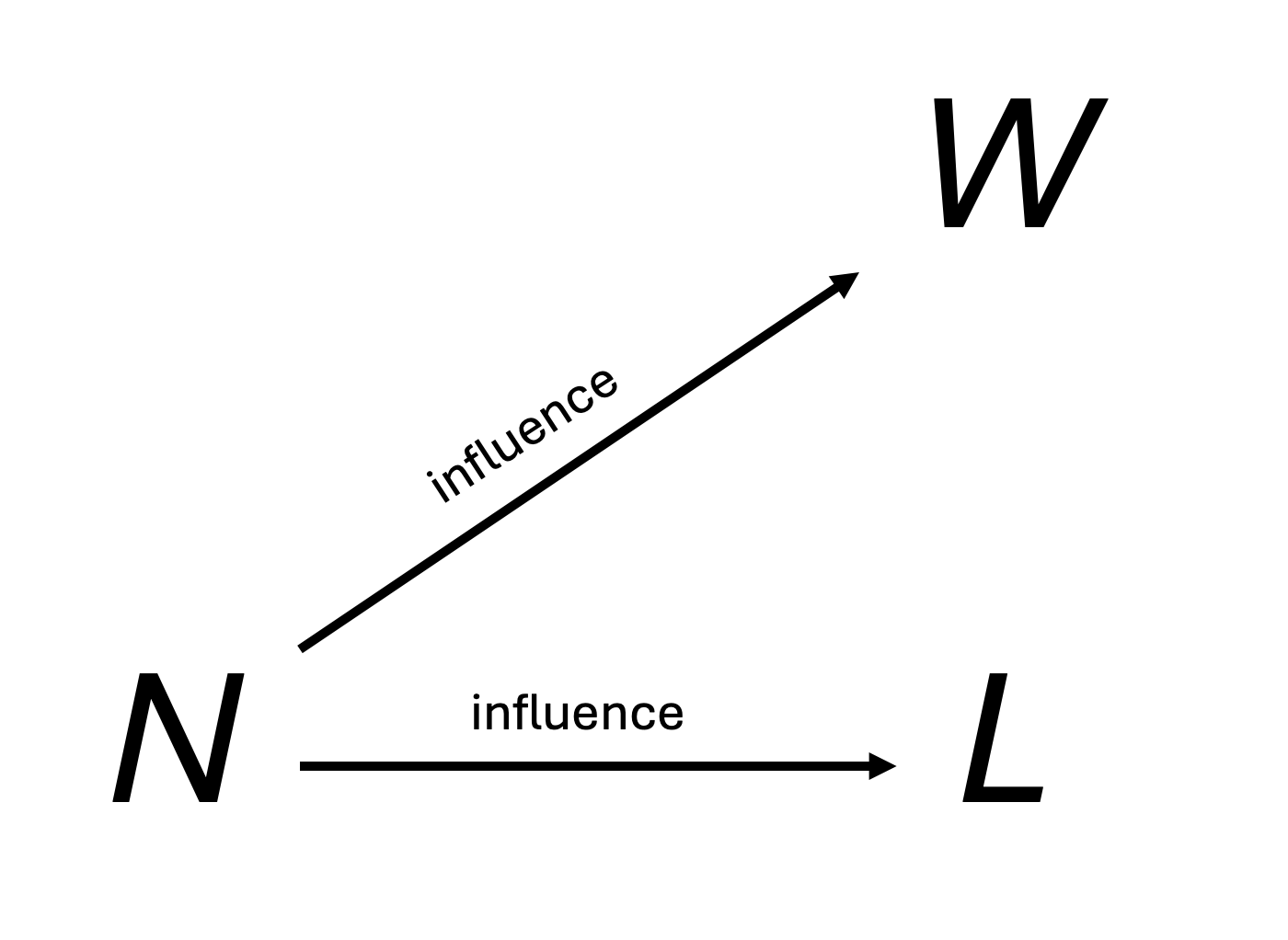
As we’ve just stated, the number of tosses of the globe \(N\) influences the number of times we see water \(W\) or land \(L\) because the more times we toss the globe, the larger \(W\) and \(L\) can be (and this is independent of the actual proportion of water to land). The influence of \(N\) on \(W\) and \(L\) can be described as in Figure 26.1.
The arrows in Figure 26.1 represent a causal influence of \(N\) on \(W\) and \(L\) because by varying \(N\) we can induce changes in \(W\) and/or \(L\).
But, no matter what we do to change \(W\) or \(L\) (such as faking our data, or miscounting) this does not change \(N\).
The arrows represent the consequence of intervening on the experiment by changing \(N\).

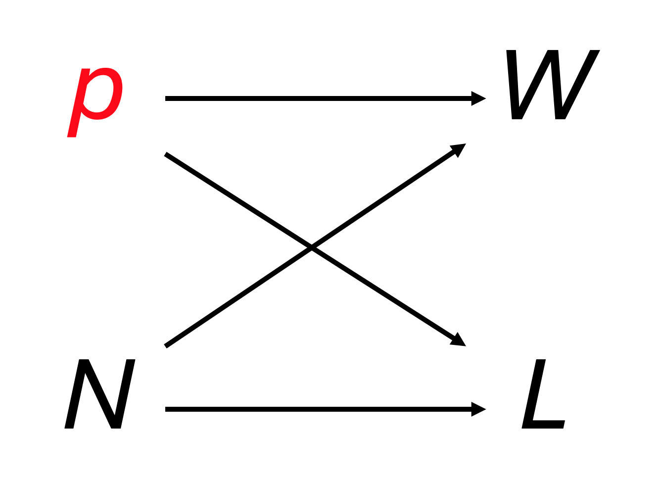
Similarly, the variable \(p\) influences \(W\) and \(L\) (Figure 26.2) because if there’s more water on the Earth’s surface \(W\) will be larger, and if there’s less water then \(L\) will be larger.
We can’t vary \(p\) in practice, but we can imaging creating a new continent in the middle of the Atlantic, say, and thus decreasing the proportion of the Earth’s surface that is water. That would be an intervention on the experiment that we can consider but not implement. We could predict the consequence of making a change even if we can’t make that change in practice.
Again, the arrows in Figure 26.2 represent a causal influence of \(p\) on \(W\) and \(L\) because - in principle - by varying \(p\) we can induce changes in \(W\) and/or \(L\).
Again, no matter what we do to change \(W\) or \(L\) (such as faking our data, or miscounting) this does not change \(p\).
The arrows represent the consequence of intervening on the experiment by changing \(p\) (not that we can actually do this, in practice).

26.3 What the graph tells us
The graph in Figure 26.2 represents our scientific knowledge about the system. It shows that we understand:
- The actual proportion of water \(p\) on the surface of the Earth affects our measured values \(W\) and \(L\)
- The number of times we make a measurement (spin the globe) \(N\) affects our measured values \(W\) and \(L\)
There is no arrow linking \(W\) to \(L\), or \(L\) to \(W\). This implies that the two measurements do not influence each other: they are independent measurements.
This means that we assume that we have the same probability of observation a W or an L, regardless of what the previous observation was. (This may not be true in all experiments, and your experimental design needs to take that into account, if it is the case).
The graph does not tell us exactly how either \(p\) or \(N\) affect the values of \(W\) and \(L\).
However, in this simple system, the nature of the relationships is intuitive:
- every time we toss the globe we take a new measurement and increase either \(W\) or \(L\) by one
- the actual proportion of water on the globe’s surface should be reflected in the relative counts of \(W\) and \(L\)
It is good practice, for every experiment that you do, to draw out what you understand about the causal relationships in the experiment.
Drawing these graphs can help you understand your experiments better, and develop effective experimental designs. Considering these structures can identify good (and bad) controls for your experiments.
Now that we have considered the causal structure of our model, we can start to analyse the data from Figure 25.3.
This is essentially saying that you are incorporating what you understand of cause and effect into the way the experiment works. We will return to the ideas cause and effect, shortly.↩︎
This is similar to the situation where we estimate the effect of a drug (in a general population) by observing it indirectly in a sample drawn from that population.↩︎